in single subject research unstable data

An official website of the United States government

The .gov means it’s official. Federal government websites often end in .gov or .mil. Before sharing sensitive information, make sure you’re on a federal government site.

The site is secure. The https:// ensures that you are connecting to the official website and that any information you provide is encrypted and transmitted securely.

Publications
Account settings
My Bibliography
Collections
Citation manager

Save citation to file

Email citation, add to collections.

Create a new collection
Add to an existing collection

Add to My Bibliography

Your saved search, create a file for external citation management software, your rss feed.

Search in PubMed
Search in NLM Catalog
Add to Search

The statistical analysis of single-subject data: a comparative examination

Affiliation.

1 Therapeutic Science Program, University of Wisconsin-Madison.
PMID: 8047564
DOI: 10.1093/ptj/74.8.768

Background and purpose: The purposes of this study were to examine whether the use of three different statistical methods for analyzing single-subject data led to similar results and to identify components of graphed data that influence agreement (or disagreement) among the statistical procedures.

Methods: Forty-two graphs containing single-subject data were examined. Twenty-one were AB charts of hypothetical data. The other 21 graphs appeared in Journal of Applied Behavioral Analysis, Physical Therapy, Journal of the Association for Persons With Severe Handicaps, and Journal of Behavior Therapy and Experimental Psychiatry. Three different statistical tests--the C statistic, the two-standard deviation band method, and the split-middle method of trend estimation--were used to analyze the 42 graphs.

Results: A relatively low degree of agreement (38%) was found among the three statistical tests. The highest rate of agreement for any two statistical procedures (71%) was found for the two-standard deviation band method and the C statistic. A logistic regression analysis revealed that overlap in single-subject graphed data was the best predictor of disagreement among the three statistical tests (beta = .49, P < .03).

Conclusion and discussion: The results indicate that interpretation of data from single-subject research designs is directly influenced by the method of data analysis selected. Variation exists across both visual and statistical methods of data reduction. The advantages and disadvantages of statistical and visual analysis are described.

PubMed Disclaimer

Statistical analysis of single-subject designs. Janosky JE, Al-shboul Q. Janosky JE, et al. Phys Ther. 1995 Feb;75(2):157-8. doi: 10.1093/ptj/75.2.157. Phys Ther. 1995. PMID: 7846136 No abstract available.

Publication types

Search in MeSH

LinkOut - more resources

Full text sources.

Silverchair Information Systems

Citation Manager

NCBI Literature Resources

MeSH PMC Bookshelf Disclaimer

The PubMed wordmark and PubMed logo are registered trademarks of the U.S. Department of Health and Human Services (HHS). Unauthorized use of these marks is strictly prohibited.

Want to create or adapt books like this? Learn more about how Pressbooks supports open publishing practices.

45 Single-Subject Research Designs

Learning objectives.

Describe the basic elements of a single-subject research design.
Design simple single-subject studies using reversal and multiple-baseline designs.
Explain how single-subject research designs address the issue of internal validity.
Interpret the results of simple single-subject studies based on the visual inspection of graphed data.

General Features of Single-Subject Designs

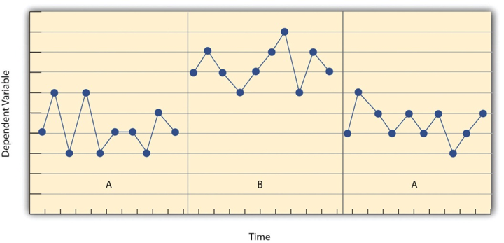
Before looking at any specific single-subject research designs, it will be helpful to consider some features that are common to most of them. Many of these features are illustrated in Figure 10.1, which shows the results of a generic single-subject study. First, the dependent variable (represented on the y -axis of the graph) is measured repeatedly over time (represented by the x -axis) at regular intervals. Second, the study is divided into distinct phases, and the participant is tested under one condition per phase. The conditions are often designated by capital letters: A, B, C, and so on. Thus Figure 10.1 represents a design in which the participant was tested first in one condition (A), then tested in another condition (B), and finally retested in the original condition (A). (This is called a reversal design and will be discussed in more detail shortly.)

Figure 10.2 Results of a Generic Single-Subject Study Illustrating Several Principles of Single-Subject Research

Another important aspect of single-subject research is that the change from one condition to the next does not usually occur after a fixed amount of time or number of observations. Instead, it depends on the participant’s behavior. Specifically, the researcher waits until the participant’s behavior in one condition becomes fairly consistent from observation to observation before changing conditions. This is sometimes referred to as the steady state strategy (Sidman, 1960) [1] . The idea is that when the dependent variable has reached a steady state, then any change across conditions will be relatively easy to detect. Recall that we encountered this same principle when discussing experimental research more generally. The effect of an independent variable is easier to detect when the “noise” in the data is minimized.

Reversal Designs

The most basic single-subject research design is the reversal design , also called the ABA design . During the first phase, A, a baseline is established for the dependent variable. This is the level of responding before any treatment is introduced, and therefore the baseline phase is a kind of control condition. When steady state responding is reached, phase B begins as the researcher introduces the treatment. There may be a period of adjustment to the treatment during which the behavior of interest becomes more variable and begins to increase or decrease. Again, the researcher waits until that dependent variable reaches a steady state so that it is clear whether and how much it has changed. Finally, the researcher removes the treatment and again waits until the dependent variable reaches a steady state. This basic reversal design can also be extended with the reintroduction of the treatment (ABAB), another return to baseline (ABABA), and so on.

The study by Hall and his colleagues employed an ABAB reversal design. Figure 10.2 approximates the data for Robbie. The percentage of time he spent studying (the dependent variable) was low during the first baseline phase, increased during the first treatment phase until it leveled off, decreased during the second baseline phase, and again increased during the second treatment phase.

Figure 10.3 An Approximation of the Results for Hall and Colleagues’ Participant Robbie in Their ABAB Reversal Design

Why is the reversal—the removal of the treatment—considered to be necessary in this type of design? Why use an ABA design, for example, rather than a simpler AB design? Notice that an AB design is essentially an interrupted time-series design applied to an individual participant. Recall that one problem with that design is that if the dependent variable changes after the treatment is introduced, it is not always clear that the treatment was responsible for the change. It is possible that something else changed at around the same time and that this extraneous variable is responsible for the change in the dependent variable. But if the dependent variable changes with the introduction of the treatment and then changes back with the removal of the treatment (assuming that the treatment does not create a permanent effect), it is much clearer that the treatment (and removal of the treatment) is the cause. In other words, the reversal greatly increases the internal validity of the study.

There are close relatives of the basic reversal design that allow for the evaluation of more than one treatment. In a multiple-treatment reversal design , a baseline phase is followed by separate phases in which different treatments are introduced. For example, a researcher might establish a baseline of studying behavior for a disruptive student (A), then introduce a treatment involving positive attention from the teacher (B), and then switch to a treatment involving mild punishment for not studying (C). The participant could then be returned to a baseline phase before reintroducing each treatment—perhaps in the reverse order as a way of controlling for carryover effects. This particular multiple-treatment reversal design could also be referred to as an ABCACB design.

In an alternating treatments design , two or more treatments are alternated relatively quickly on a regular schedule. For example, positive attention for studying could be used one day and mild punishment for not studying the next, and so on. Or one treatment could be implemented in the morning and another in the afternoon. The alternating treatments design can be a quick and effective way of comparing treatments, but only when the treatments are fast acting.

Multiple-Baseline Designs

There are two potential problems with the reversal design—both of which have to do with the removal of the treatment. One is that if a treatment is working, it may be unethical to remove it. For example, if a treatment seemed to reduce the incidence of self-injury in a child with an intellectual delay, it would be unethical to remove that treatment just to show that the incidence of self-injury increases. The second problem is that the dependent variable may not return to baseline when the treatment is removed. For example, when positive attention for studying is removed, a student might continue to study at an increased rate. This could mean that the positive attention had a lasting effect on the student’s studying, which of course would be good. But it could also mean that the positive attention was not really the cause of the increased studying in the first place. Perhaps something else happened at about the same time as the treatment—for example, the student’s parents might have started rewarding him for good grades. One solution to these problems is to use a multiple-baseline design , which is represented in Figure 10.3. There are three different types of multiple-baseline designs which we will now consider.

Multiple-Baseline Design Across Participants

In one version of the design, a baseline is established for each of several participants, and the treatment is then introduced for each one. In essence, each participant is tested in an AB design. The key to this design is that the treatment is introduced at a different time for each participant. The idea is that if the dependent variable changes when the treatment is introduced for one participant, it might be a coincidence. But if the dependent variable changes when the treatment is introduced for multiple participants—especially when the treatment is introduced at different times for the different participants—then it is unlikely to be a coincidence.

Figure 10.4 Results of a Generic Multiple-Baseline Study. The multiple baselines can be for different participants, dependent variables, or settings. The treatment is introduced at a different time on each baseline.

As an example, consider a study by Scott Ross and Robert Horner (Ross & Horner, 2009) [2] . They were interested in how a school-wide bullying prevention program affected the bullying behavior of particular problem students. At each of three different schools, the researchers studied two students who had regularly engaged in bullying. During the baseline phase, they observed the students for 10-minute periods each day during lunch recess and counted the number of aggressive behaviors they exhibited toward their peers. After 2 weeks, they implemented the program at one school. After 2 more weeks, they implemented it at the second school. And after 2 more weeks, they implemented it at the third school. They found that the number of aggressive behaviors exhibited by each student dropped shortly after the program was implemented at the student’s school. Notice that if the researchers had only studied one school or if they had introduced the treatment at the same time at all three schools, then it would be unclear whether the reduction in aggressive behaviors was due to the bullying program or something else that happened at about the same time it was introduced (e.g., a holiday, a television program, a change in the weather). But with their multiple-baseline design, this kind of coincidence would have to happen three separate times—a very unlikely occurrence—to explain their results.

Multiple-Baseline Design Across Behaviors

In another version of the multiple-baseline design, multiple baselines are established for the same participant but for different dependent variables, and the treatment is introduced at a different time for each dependent variable. Imagine, for example, a study on the effect of setting clear goals on the productivity of an office worker who has two primary tasks: making sales calls and writing reports. Baselines for both tasks could be established. For example, the researcher could measure the number of sales calls made and reports written by the worker each week for several weeks. Then the goal-setting treatment could be introduced for one of these tasks, and at a later time the same treatment could be introduced for the other task. The logic is the same as before. If productivity increases on one task after the treatment is introduced, it is unclear whether the treatment caused the increase. But if productivity increases on both tasks after the treatment is introduced—especially when the treatment is introduced at two different times—then it seems much clearer that the treatment was responsible.

Multiple-Baseline Design Across Settings

In yet a third version of the multiple-baseline design, multiple baselines are established for the same participant but in different settings. For example, a baseline might be established for the amount of time a child spends reading during his free time at school and during his free time at home. Then a treatment such as positive attention might be introduced first at school and later at home. Again, if the dependent variable changes after the treatment is introduced in each setting, then this gives the researcher confidence that the treatment is, in fact, responsible for the change.

Data Analysis in Single-Subject Research

In addition to its focus on individual participants, single-subject research differs from group research in the way the data are typically analyzed. As we have seen throughout the book, group research involves combining data across participants. Group data are described using statistics such as means, standard deviations, correlation coefficients, and so on to detect general patterns. Finally, inferential statistics are used to help decide whether the result for the sample is likely to generalize to the population. Single-subject research, by contrast, relies heavily on a very different approach called visual inspection . This means plotting individual participants’ data as shown throughout this chapter, looking carefully at those data, and making judgments about whether and to what extent the independent variable had an effect on the dependent variable. Inferential statistics are typically not used.

In visually inspecting their data, single-subject researchers take several factors into account. One of them is changes in the level of the dependent variable from condition to condition. If the dependent variable is much higher or much lower in one condition than another, this suggests that the treatment had an effect. A second factor is trend , which refers to gradual increases or decreases in the dependent variable across observations. If the dependent variable begins increasing or decreasing with a change in conditions, then again this suggests that the treatment had an effect. It can be especially telling when a trend changes directions—for example, when an unwanted behavior is increasing during baseline but then begins to decrease with the introduction of the treatment. A third factor is latency , which is the time it takes for the dependent variable to begin changing after a change in conditions. In general, if a change in the dependent variable begins shortly after a change in conditions, this suggests that the treatment was responsible.

In the top panel of Figure 10.4, there are fairly obvious changes in the level and trend of the dependent variable from condition to condition. Furthermore, the latencies of these changes are short; the change happens immediately. This pattern of results strongly suggests that the treatment was responsible for the changes in the dependent variable. In the bottom panel of Figure 10.4, however, the changes in level are fairly small. And although there appears to be an increasing trend in the treatment condition, it looks as though it might be a continuation of a trend that had already begun during baseline. This pattern of results strongly suggests that the treatment was not responsible for any changes in the dependent variable—at least not to the extent that single-subject researchers typically hope to see.

Figure 10.5 Results of a Generic Single-Subject Study Illustrating Level, Trend, and Latency. Visual inspection of the data suggests an effective treatment in the top panel but an ineffective treatment in the bottom panel.

The results of single-subject research can also be analyzed using statistical procedures—and this is becoming more common. There are many different approaches, and single-subject researchers continue to debate which are the most useful. One approach parallels what is typically done in group research. The mean and standard deviation of each participant’s responses under each condition are computed and compared, and inferential statistical tests such as the t test or analysis of variance are applied (Fisch, 2001) [3] . (Note that averaging across participants is less common.) Another approach is to compute the percentage of non-overlapping data (PND) for each participant (Scruggs & Mastropieri, 2001) [4] . This is the percentage of responses in the treatment condition that are more extreme than the most extreme response in a relevant control condition. In the study of Hall and his colleagues, for example, all measures of Robbie’s study time in the first treatment condition were greater than the highest measure in the first baseline, for a PND of 100%. The greater the percentage of non-overlapping data, the stronger the treatment effect. Still, formal statistical approaches to data analysis in single-subject research are generally considered a supplement to visual inspection, not a replacement for it.

Sidman, M. (1960). Tactics of scientific research: Evaluating experimental data in psychology . Boston, MA: Authors Cooperative. ↵
Ross, S. W., & Horner, R. H. (2009). Bully prevention in positive behavior support. Journal of Applied Behavior Analysis, 42 , 747–759. ↵
Fisch, G. S. (2001). Evaluating data from behavioral analysis: Visual inspection or statistical models. Behavioral Processes, 54 , 137–154. ↵
Scruggs, T. E., & Mastropieri, M. A. (2001). How to summarize single-participant research: Ideas and applications. Exceptionality, 9 , 227–244. ↵

The most basic single-subject research design in which the researcher measures the dependent variable in three phases: Baseline, before a treatment is introduced (A); after the treatment is introduced (B); and then a return to baseline after removing the treatment (A). It is often called an ABA design.

Another term for reversal design.

This means plotting individual participants’ data, looking carefully at those plots, and making judgments about whether and to what extent the independent variable had an effect on the dependent variable.

This is the percentage of responses in the treatment condition that are more extreme than the most extreme response in a relevant control condition.

Research Methods in Psychology Copyright © 2019 by Rajiv S. Jhangiani, I-Chant A. Chiang, Carrie Cuttler, & Dana C. Leighton is licensed under a Creative Commons Attribution-NonCommercial-ShareAlike 4.0 International License , except where otherwise noted.

Share This Book

10.2 Single-Subject Research Designs

Learning objectives.

Describe the basic elements of a single-subject research design.
Design simple single-subject studies using reversal and multiple-baseline designs.
Explain how single-subject research designs address the issue of internal validity.
Interpret the results of simple single-subject studies based on the visual inspection of graphed data.

General Features of Single-Subject Designs

Figure 10.1 Results of a Generic Single-Subject Study Illustrating Several Principles of Single-Subject Research

Reversal Designs

Figure 10.2 An Approximation of the Results for Hall and Colleagues’ Participant Robbie in Their ABAB Reversal Design

Multiple-Baseline Designs

Multiple-Baseline Design Across Participants

Figure 10.3 Results of a Generic Multiple-Baseline Study. The multiple baselines can be for different participants, dependent variables, or settings. The treatment is introduced at a different time on each baseline.

As an example, consider a study by Scott Ross and Robert Horner (Ross & Horner, 2009) [2] . They were interested in how a school-wide bullying prevention program affected the bullying behavior of particular problem students. At each of three different schools, the researchers studied two students who had regularly engaged in bullying. During the baseline phase, they observed the students for 10-minute periods each day during lunch recess and counted the number of aggressive behaviors they exhibited toward their peers. After 2 weeks, they implemented the program at one school. After 2 more weeks, they implemented it at the second school. And after 2 more weeks, they implemented it at the third school. They found that the number of aggressive behaviors exhibited by each student dropped shortly after the program was implemented at his or her school. Notice that if the researchers had only studied one school or if they had introduced the treatment at the same time at all three schools, then it would be unclear whether the reduction in aggressive behaviors was due to the bullying program or something else that happened at about the same time it was introduced (e.g., a holiday, a television program, a change in the weather). But with their multiple-baseline design, this kind of coincidence would have to happen three separate times—a very unlikely occurrence—to explain their results.

Multiple-Baseline Design Across Behaviors

Multiple-Baseline Design Across Settings

Data Analysis in Single-Subject Research

Figure 10.4 Results of a Generic Single-Subject Study Illustrating Level, Trend, and Latency. Visual inspection of the data suggests an effective treatment in the top panel but an ineffective treatment in the bottom panel.

Key Takeaways

Single-subject research designs typically involve measuring the dependent variable repeatedly over time and changing conditions (e.g., from baseline to treatment) when the dependent variable has reached a steady state. This approach allows the researcher to see whether changes in the independent variable are causing changes in the dependent variable.
In a reversal design, the participant is tested in a baseline condition, then tested in a treatment condition, and then returned to baseline. If the dependent variable changes with the introduction of the treatment and then changes back with the return to baseline, this provides strong evidence of a treatment effect.
In a multiple-baseline design, baselines are established for different participants, different dependent variables, or different settings—and the treatment is introduced at a different time on each baseline. If the introduction of the treatment is followed by a change in the dependent variable on each baseline, this provides strong evidence of a treatment effect.
Single-subject researchers typically analyze their data by graphing them and making judgments about whether the independent variable is affecting the dependent variable based on level, trend, and latency.
Does positive attention from a parent increase a child’s tooth-brushing behavior?
Does self-testing while studying improve a student’s performance on weekly spelling tests?
Does regular exercise help relieve depression?
Practice: Create a graph that displays the hypothetical results for the study you designed in Exercise 1. Write a paragraph in which you describe what the results show. Be sure to comment on level, trend, and latency.
Sidman, M. (1960). Tactics of scientific research: Evaluating experimental data in psychology . Boston, MA: Authors Cooperative. ↵
Ross, S. W., & Horner, R. H. (2009). Bully prevention in positive behavior support. Journal of Applied Behavior Analysis, 42 , 747–759. ↵
Fisch, G. S. (2001). Evaluating data from behavioral analysis: Visual inspection or statistical models. Behavioral Processes, 54 , 137–154. ↵
Scruggs, T. E., & Mastropieri, M. A. (2001). How to summarize single-participant research: Ideas and applications. Exceptionality, 9 , 227–244. ↵

Share This Book

Increase Font Size

Want to create or adapt books like this? Learn more about how Pressbooks supports open publishing practices.

Single-Subject Research Designs

Rajiv S. Jhangiani; I-Chant A. Chiang; Carrie Cuttler; and Dana C. Leighton

Learning Objectives

Describe the basic elements of a single-subject research design.
Design simple single-subject studies using reversal and multiple-baseline designs.
Explain how single-subject research designs address the issue of internal validity.
Interpret the results of simple single-subject studies based on the visual inspection of graphed data.

General Features of Single-Subject Designs

in single subject research unstable data

Reversal Designs

ABAB Reversal Design. Image description available.

Multiple-Baseline Designs

Multiple-Baseline Design Across Participants

Results of a Generic Multiple-Baseline Study. Image description available.

Multiple-Baseline Design Across Behaviors

Multiple-Baseline Design Across Settings

Data Analysis in Single-Subject Research

Image Description

Figure 10.2 long description: Line graph showing the results of a study with an ABAB reversal design. The dependent variable was low during first baseline phase; increased during the first treatment; decreased during the second baseline, but was still higher than during the first baseline; and was highest during the second treatment phase. [Return to Figure 10.2]

Figure 10.3 long description: Three line graphs showing the results of a generic multiple-baseline study, in which different baselines are established and treatment is introduced to participants at different times.

For Baseline 1, treatment is introduced one-quarter of the way into the study. The dependent variable ranges between 12 and 16 units during the baseline, but drops down to 10 units with treatment and mostly decreases until the end of the study, ranging between 4 and 10 units.

For Baseline 2, treatment is introduced halfway through the study. The dependent variable ranges between 10 and 15 units during the baseline, then has a sharp decrease to 7 units when treatment is introduced. However, the dependent variable increases to 12 units soon after the drop and ranges between 8 and 10 units until the end of the study.

For Baseline 3, treatment is introduced three-quarters of the way into the study. The dependent variable ranges between 12 and 16 units for the most part during the baseline, with one drop down to 10 units. When treatment is introduced, the dependent variable drops down to 10 units and then ranges between 8 and 9 units until the end of the study. [Return to Figure 10.3]

Figure 10.4 long description: Two graphs showing the results of a generic single-subject study with an ABA design. In the first graph, under condition A, level is high and the trend is increasing. Under condition B, level is much lower than under condition A and the trend is decreasing. Under condition A again, level is about as high as the first time and the trend is increasing. For each change, latency is short, suggesting that the treatment is the reason for the change.

In the second graph, under condition A, level is relatively low and the trend is increasing. Under condition B, level is a little higher than during condition A and the trend is increasing slightly. Under condition A again, level is a little lower than during condition B and the trend is decreasing slightly. It is difficult to determine the latency of these changes, since each change is rather minute, which suggests that the treatment is ineffective. [Return to Figure 10.4]

Sidman, M. (1960). Tactics of scientific research: Evaluating experimental data in psychology . Boston, MA: Authors Cooperative. ↵
Ross, S. W., & Horner, R. H. (2009). Bully prevention in positive behavior support. Journal of Applied Behavior Analysis, 42 , 747–759. ↵
Fisch, G. S. (2001). Evaluating data from behavioral analysis: Visual inspection or statistical models. Behavioral Processes, 54 , 137–154. ↵
Scruggs, T. E., & Mastropieri, M. A. (2001). How to summarize single-participant research: Ideas and applications. Exceptionality, 9 , 227–244. ↵

When the researcher waits until the participant’s behavior in one condition becomes fairly consistent from observation to observation before changing conditions.

Another term for reversal design.

The beginning phase of an ABA design which acts as a kind of control condition in which the level of responding before any treatment is introduced.

In this design the baseline phase is followed by separate phases in which different treatments are introduced.

In this design two or more treatments are alternated relatively quickly on a regular schedule.

In this design, multiple baselines are either established for one participant or one baseline is established for many participants.

This is the percentage of responses in the treatment condition that are more extreme than the most extreme response in a relevant control condition.

Single-Subject Research Designs Copyright © by Rajiv S. Jhangiani; I-Chant A. Chiang; Carrie Cuttler; and Dana C. Leighton is licensed under a Creative Commons Attribution-NonCommercial-ShareAlike 4.0 International License , except where otherwise noted.

Share This Book

Want to create or adapt books like this? Learn more about how Pressbooks supports open publishing practices.

Chapter 10: Single-Subject Research

Single-Subject Research Designs

Learning Objectives

Describe the basic elements of a single-subject research design.
Design simple single-subject studies using reversal and multiple-baseline designs.
Explain how single-subject research designs address the issue of internal validity.
Interpret the results of simple single-subject studies based on the visual inspection of graphed data.

General Features of Single-Subject Designs

Before looking at any specific single-subject research designs, it will be helpful to consider some features that are common to most of them. Many of these features are illustrated in Figure 10.2, which shows the results of a generic single-subject study. First, the dependent variable (represented on the y -axis of the graph) is measured repeatedly over time (represented by the x -axis) at regular intervals. Second, the study is divided into distinct phases, and the participant is tested under one condition per phase. The conditions are often designated by capital letters: A, B, C, and so on. Thus Figure 10.2 represents a design in which the participant was tested first in one condition (A), then tested in another condition (B), and finally retested in the original condition (A). (This is called a reversal design and will be discussed in more detail shortly.)

A subject was tested under condition A, then condition B, then under condition A again.

Another important aspect of single-subject research is that the change from one condition to the next does not usually occur after a fixed amount of time or number of observations. Instead, it depends on the participant’s behaviour. Specifically, the researcher waits until the participant’s behaviour in one condition becomes fairly consistent from observation to observation before changing conditions. This is sometimes referred to as the steady state strategy (Sidman, 1960) [1] . The idea is that when the dependent variable has reached a steady state, then any change across conditions will be relatively easy to detect. Recall that we encountered this same principle when discussing experimental research more generally. The effect of an independent variable is easier to detect when the “noise” in the data is minimized.

Reversal Designs

The most basic single-subject research design is the reversal design , also called the ABA design . During the first phase, A, a baseline is established for the dependent variable. This is the level of responding before any treatment is introduced, and therefore the baseline phase is a kind of control condition. When steady state responding is reached, phase B begins as the researcher introduces the treatment. There may be a period of adjustment to the treatment during which the behaviour of interest becomes more variable and begins to increase or decrease. Again, the researcher waits until that dependent variable reaches a steady state so that it is clear whether and how much it has changed. Finally, the researcher removes the treatment and again waits until the dependent variable reaches a steady state. This basic reversal design can also be extended with the reintroduction of the treatment (ABAB), another return to baseline (ABABA), and so on.

The study by Hall and his colleagues was an ABAB reversal design. Figure 10.3 approximates the data for Robbie. The percentage of time he spent studying (the dependent variable) was low during the first baseline phase, increased during the first treatment phase until it leveled off, decreased during the second baseline phase, and again increased during the second treatment phase.

A graph showing the results of a study with an ABAB reversal design. Long description available.

There are close relatives of the basic reversal design that allow for the evaluation of more than one treatment. In a multiple-treatment reversal design , a baseline phase is followed by separate phases in which different treatments are introduced. For example, a researcher might establish a baseline of studying behaviour for a disruptive student (A), then introduce a treatment involving positive attention from the teacher (B), and then switch to a treatment involving mild punishment for not studying (C). The participant could then be returned to a baseline phase before reintroducing each treatment—perhaps in the reverse order as a way of controlling for carryover effects. This particular multiple-treatment reversal design could also be referred to as an ABCACB design.

Multiple-Baseline Designs

There are two potential problems with the reversal design—both of which have to do with the removal of the treatment. One is that if a treatment is working, it may be unethical to remove it. For example, if a treatment seemed to reduce the incidence of self-injury in a developmentally disabled child, it would be unethical to remove that treatment just to show that the incidence of self-injury increases. The second problem is that the dependent variable may not return to baseline when the treatment is removed. For example, when positive attention for studying is removed, a student might continue to study at an increased rate. This could mean that the positive attention had a lasting effect on the student’s studying, which of course would be good. But it could also mean that the positive attention was not really the cause of the increased studying in the first place. Perhaps something else happened at about the same time as the treatment—for example, the student’s parents might have started rewarding him for good grades.

One solution to these problems is to use a multiple-baseline design , which is represented in Figure 10.4. In one version of the design, a baseline is established for each of several participants, and the treatment is then introduced for each one. In essence, each participant is tested in an AB design. The key to this design is that the treatment is introduced at a different time for each participant. The idea is that if the dependent variable changes when the treatment is introduced for one participant, it might be a coincidence. But if the dependent variable changes when the treatment is introduced for multiple participants—especially when the treatment is introduced at different times for the different participants—then it is extremely unlikely to be a coincidence.

Three graphs depicting the results of a multiple-baseline study. Long description available.

As an example, consider a study by Scott Ross and Robert Horner (Ross & Horner, 2009) [2] . They were interested in how a school-wide bullying prevention program affected the bullying behaviour of particular problem students. At each of three different schools, the researchers studied two students who had regularly engaged in bullying. During the baseline phase, they observed the students for 10-minute periods each day during lunch recess and counted the number of aggressive behaviours they exhibited toward their peers. (The researchers used handheld computers to help record the data.) After 2 weeks, they implemented the program at one school. After 2 more weeks, they implemented it at the second school. And after 2 more weeks, they implemented it at the third school. They found that the number of aggressive behaviours exhibited by each student dropped shortly after the program was implemented at his or her school. Notice that if the researchers had only studied one school or if they had introduced the treatment at the same time at all three schools, then it would be unclear whether the reduction in aggressive behaviours was due to the bullying program or something else that happened at about the same time it was introduced (e.g., a holiday, a television program, a change in the weather). But with their multiple-baseline design, this kind of coincidence would have to happen three separate times—a very unlikely occurrence—to explain their results.

Data Analysis in Single-Subject Research

In addition to its focus on individual participants, single-subject research differs from group research in the way the data are typically analyzed. As we have seen throughout the book, group research involves combining data across participants. Group data are described using statistics such as means, standard deviations, Pearson’s r , and so on to detect general patterns. Finally, inferential statistics are used to help decide whether the result for the sample is likely to generalize to the population. Single-subject research, by contrast, relies heavily on a very different approach called visual inspection . This means plotting individual participants’ data as shown throughout this chapter, looking carefully at those data, and making judgments about whether and to what extent the independent variable had an effect on the dependent variable. Inferential statistics are typically not used.

In visually inspecting their data, single-subject researchers take several factors into account. One of them is changes in the level of the dependent variable from condition to condition. If the dependent variable is much higher or much lower in one condition than another, this suggests that the treatment had an effect. A second factor is trend , which refers to gradual increases or decreases in the dependent variable across observations. If the dependent variable begins increasing or decreasing with a change in conditions, then again this suggests that the treatment had an effect. It can be especially telling when a trend changes directions—for example, when an unwanted behaviour is increasing during baseline but then begins to decrease with the introduction of the treatment. A third factor is latency , which is the time it takes for the dependent variable to begin changing after a change in conditions. In general, if a change in the dependent variable begins shortly after a change in conditions, this suggests that the treatment was responsible.

In the top panel of Figure 10.5, there are fairly obvious changes in the level and trend of the dependent variable from condition to condition. Furthermore, the latencies of these changes are short; the change happens immediately. This pattern of results strongly suggests that the treatment was responsible for the changes in the dependent variable. In the bottom panel of Figure 10.5, however, the changes in level are fairly small. And although there appears to be an increasing trend in the treatment condition, it looks as though it might be a continuation of a trend that had already begun during baseline. This pattern of results strongly suggests that the treatment was not responsible for any changes in the dependent variable—at least not to the extent that single-subject researchers typically hope to see.

Results of a single-subject study showing level, trend and latency. Long description available.

The results of single-subject research can also be analyzed using statistical procedures—and this is becoming more common. There are many different approaches, and single-subject researchers continue to debate which are the most useful. One approach parallels what is typically done in group research. The mean and standard deviation of each participant’s responses under each condition are computed and compared, and inferential statistical tests such as the t test or analysis of variance are applied (Fisch, 2001) [3] . (Note that averaging across participants is less common.) Another approach is to compute the percentage of nonoverlapping data (PND) for each participant (Scruggs & Mastropieri, 2001) [4] . This is the percentage of responses in the treatment condition that are more extreme than the most extreme response in a relevant control condition. In the study of Hall and his colleagues, for example, all measures of Robbie’s study time in the first treatment condition were greater than the highest measure in the first baseline, for a PND of 100%. The greater the percentage of nonoverlapping data, the stronger the treatment effect. Still, formal statistical approaches to data analysis in single-subject research are generally considered a supplement to visual inspection, not a replacement for it.

Key Takeaways

Single-subject research designs typically involve measuring the dependent variable repeatedly over time and changing conditions (e.g., from baseline to treatment) when the dependent variable has reached a steady state. This approach allows the researcher to see whether changes in the independent variable are causing changes in the dependent variable.
In a reversal design, the participant is tested in a baseline condition, then tested in a treatment condition, and then returned to baseline. If the dependent variable changes with the introduction of the treatment and then changes back with the return to baseline, this provides strong evidence of a treatment effect.
In a multiple-baseline design, baselines are established for different participants, different dependent variables, or different settings—and the treatment is introduced at a different time on each baseline. If the introduction of the treatment is followed by a change in the dependent variable on each baseline, this provides strong evidence of a treatment effect.
Single-subject researchers typically analyze their data by graphing them and making judgments about whether the independent variable is affecting the dependent variable based on level, trend, and latency.
Does positive attention from a parent increase a child’s toothbrushing behaviour?
Does self-testing while studying improve a student’s performance on weekly spelling tests?
Does regular exercise help relieve depression?
Practice: Create a graph that displays the hypothetical results for the study you designed in Exercise 1. Write a paragraph in which you describe what the results show. Be sure to comment on level, trend, and latency.

Long Descriptions

Figure 10.3 long description: Line graph showing the results of a study with an ABAB reversal design. The dependent variable was low during first baseline phase; increased during the first treatment; decreased during the second baseline, but was still higher than during the first baseline; and was highest during the second treatment phase. [Return to Figure 10.3]

Figure 10.4 long description: Three line graphs showing the results of a generic multiple-baseline study, in which different baselines are established and treatment is introduced to participants at different times.

Figure 10.5 long description: Two graphs showing the results of a generic single-subject study with an ABA design. In the first graph, under condition A, level is high and the trend is increasing. Under condition B, level is much lower than under condition A and the trend is decreasing. Under condition A again, level is about as high as the first time and the trend is increasing. For each change, latency is short, suggesting that the treatment is the reason for the change.

Sidman, M. (1960). Tactics of scientific research: Evaluating experimental data in psychology . Boston, MA: Authors Cooperative. ↵
Ross, S. W., & Horner, R. H. (2009). Bully prevention in positive behaviour support. Journal of Applied Behaviour Analysis, 42 , 747–759. ↵
Fisch, G. S. (2001). Evaluating data from behavioural analysis: Visual inspection or statistical models. Behavioural Processes, 54 , 137–154. ↵
Scruggs, T. E., & Mastropieri, M. A. (2001). How to summarize single-participant research: Ideas and applications. Exceptionality, 9 , 227–244. ↵

The researcher waits until the participant’s behaviour in one condition becomes fairly consistent from observation to observation before changing conditions. This way, any change across conditions will be easy to detect.

A study method in which the researcher gathers data on a baseline state, introduces the treatment and continues observation until a steady state is reached, and finally removes the treatment and observes the participant until they return to a steady state.

The level of responding before any treatment is introduced and therefore acts as a kind of control condition.

A baseline phase is followed by separate phases in which different treatments are introduced.

Two or more treatments are alternated relatively quickly on a regular schedule.

A baseline is established for several participants and the treatment is then introduced to each participant at a different time.

The plotting of individual participants’ data, examining the data, and making judgements about whether and to what extent the independent variable had an effect on the dependent variable.

Whether the data is higher or lower based on a visual inspection of the data; a change in the level implies the treatment introduced had an effect.

The gradual increases or decreases in the dependent variable across observations.

The time it takes for the dependent variable to begin changing after a change in conditions.

The percentage of responses in the treatment condition that are more extreme than the most extreme response in a relevant control condition.

Research Methods in Psychology - 2nd Canadian Edition Copyright © 2015 by Paul C. Price, Rajiv Jhangiani, & I-Chant A. Chiang is licensed under a Creative Commons Attribution-NonCommercial-ShareAlike 4.0 International License , except where otherwise noted.

Share This Book

Search form

You are here.

Data Analysis in Single-Subject Research

In addition to its focus on individual participants, single-subject research differs from group research in the way the data are typically analyzed. As we have seen throughout the book, group research involves combining data across participants. Group data are described using statistics such as means, standard deviations, Pearson’s r , and so on to detect general patterns. Finally, inferential statistics are used to help decide whether the result for the sample is likely to generalize to the population. Single-subject research, by contrast, relies heavily on a very different approach called v i s u a l in spe ct i o n . This means plotting individual participants’ data as shown throughout this chapter, looking carefully at those data, and making judgments about whether and to what extent the independent variable had an effect on the dependent variable. Inferential statistics are typically not used.

In visually inspecting their data, single-subject researchers take several factors into account. One of them is changes in the l e v e l of the dependent variable from condition to condition. If the dependent variable is much higher or much lower in one condition than another, this suggests that the treatment had an effect. A second factor is t r e n d , which refers to gradual increases or decreases in the dependent variable across observations. If the dependent variable begins increasing or decreasing with a change in conditions, then again this suggests that the treatment had an effect. It can be especially telling when a trend changes directions—for example, when an unwanted behavior is increasing during baseline but then begins to decrease with the introduction of the treatment. A third factor is l a t e n c y , which is the time it takes for the dependent variable to begin changing after a change in conditions. In general, if a change in the dependent variable begins shortly after a change in conditions, this suggests that the treatment was responsible.

In the top panel of Figure 10.5 , there are fairly obvious changes in the level and trend of the dependent variable from condition to condition. Furthermore, the latencies of these changes are short; the change happens immediately. This pattern of results strongly suggests that the treatment was responsible for the changes in the dependent variable. In the bottom panel of Figure 10.5 , however, the changes in level are fairly small. And although there appears to be an increasing trend in the treatment condition, it looks as though it might be a continuation of a trend that had already begun during baseline. This pattern of results strongly suggests that the treatment was not responsible for any changes in the dependent variable—at least not to the extent that single-subject researchers typically hope to see.

The results of single-subject research can also be analyzed using statistical procedures—and this is becoming more common. There are many different approaches, and single-subject researchers continue to debate which are the most useful. One approach parallels what is typically done in group research. The mean and standard deviation of each participant’s responses under each condition are computed and compared, and inferential statistical tests such as the t test or analysis of variance are applied (Fisch, 2001). 1 (Note that averaging ac r os s participants is less common.) Another approach is to compute the p e r c e n t a ge o f n o n o v e r l a ppi ng d a t a (PND) for each participant (Scruggs & Mastropieri, 2001). 2 This is the percentage of responses in the treatment condition that are more extreme than the most extreme response in a relevant control condition. In the study of Hall and his colleagues, for example, all measures of Robbie’s study time in the first treatment condition were greater than the highest measure in the first baseline, for a PND of 100%. The greater the percentage of nonoverlapping data, the stronger the treatment effect. Still, formal statistical approaches to data analysis in single-subject research are generally considered a supplement to visual inspection, not a replacement for it.

KEY TAKEAWAYS

Single-subject research designs typically involve measuring the dependent variable repeatedly over time and changing conditions (e.g., from baseline to treatment) when the dependent variable has reached a steady state. This approach allows the researcher to see whether changes in the independent variable are causing changes in the dependent variable.
In a reversal design, the participant is tested in a baseline condition, then tested in a treatment condition, and then returned to baseline. If the dependent variable changes with the introduction of the treatment and then changes back with the return to baseline, this provides strong evidence of a treatment effect.
In a multiple-baseline design, baselines are established for different participants, different dependent variables, or different settings—and the treatment is introduced at a different time on each baseline. If the introduction of the treatment is followed by a change in the dependent variable on each baseline, this provides strong evidence of a treatment effect.
Single-subject researchers typically analyze their data by graphing them and making judgments about whether the independent variable is affecting the dependent variable based on level, trend, and latency.
Does positive attention from a parent increase a child’s toothbrushing behavior?
Does self-testing while studying improve a student’s performance on weekly spelling tests?
Does regular exercise help relieve depression?Practice: Create a graph that displays the hypothetical results for the study you designed in Exercise
Write a paragraph in which you describe what the results show. Be sure to comment on level, trend, and latency.
What Is Science?
Features of Science
Science Versus Pseudoscience The Skeptic’s Dictionary KEY TAKEAWAYS EXERCISES
A Model of Scientific Research in Psychology
Who Conducts Scientific Research in Psychology? Scientific Psychology Blogs
The Broader Purposes of Scientific Research in Psychology KEY TAKEAWAYS EXERCISES
Can We Rely on Common Sense? Some Great Myths
How Could We Be So Wrong? KEY TAKEAWAYS EXERCISE
Science and Clinical Practice LEARNING OBJECTIVES Empirically Supported Treatments KEY TAKEAWAYS E X ER C IS ES
Sampling and Measurement
Differences Between Groups
Correlations Between Quantitative Variables
Correlation Does Not Imply Causation “Lots of Candy Could Lead to Violence” KEY TAKEAWAYS EXERCISE
Finding Inspiration
Generating Empirically Testable Research Questions
Interestingness
Feasibility KEY TAKEAWAYS EXERCISE
Professional Journals
Scholarly Books
Using PsycINFO and Other Databases
Using Other Search Techniques
What to Search For KEY TAKEAWAYS EXERCISE
A Framework for Thinking About Research Ethics
Weighing Risks Against Benefits Was It Worth It?
Acting Responsibly and With Integrity
Seeking Justice “They Were Betrayed”
Respecting People’s Rights and Dignity
Unavoidable Ethical Conflict KEY TAKEAWAYS EXERCISE
Historical Overview Ethics Codes
Informed Consent
Nonhuman Animal Subjects
Scholarly Integrity KEY TAKEAWAYS EXERCISES
Know and Accept Your Ethical Responsibilities
Identify and Minimize Risks
Identify and Minimize Deception
Weigh the Risks Against the Benefits
Create Informed Consent and Debriefing Procedures
Get Approval
Follow Through KEY TAKEAWAYS EXERCISES
Phenomena Some Famous Psychological Phenomena
What Is a Theory?
What Are Theories For?
Organization
Generation of New Research
Multiple Theories Where Do Multiple Personalities Come From? KEY TAKEAWAYS EXERCISES
Formality Formal Theories in Psychology
Theoretical Approach KEY TAKEAWAY EXERCISE
Constructing or Choosing a Theory
Deriving Hypotheses
Evaluating and Revising Theories
Incorporating Theory Into Your Research KEY TAKEAWAYS EXERCISE
What Is Measurement?
Psychological Constructs The Big Five
Operational Definitions
Levels of Measurement KEY TAKEAWAYS EXERCISES
Test-Retest Reliability
Internal Consistency
Interrater Reliability
Face Validity How Prejudiced Are You?
Content Validity
Criterion Validity
Discriminant Validity KEY TAKEAWAYS EXERCISES
Conceptually Defining the Construct
Using an Existing Measure
Creating Your Own Measure
Implementing the Measure
Evaluating the Measure KEY TAKEAWAYS EXERCISES
What Is an Experiment?
Internal Validity
External Validity
Manipulation of the Independent Variable
Extraneous Variables as “Noise”
Extraneous Variables as Confounding Variables KEY TAKEAWAYS EXERCISES
Random Assignment
Treatment and Control Conditions The Powerful Placebo
Carryover Effects and Counterbalancing When 9 Is “Larger” Than 221
Simultaneous Within-Subjects Designs
Between-Subjects or Within-Subjects? KEY TAKEAWAYS EXERCISES
Recruiting Participants The Volunteer Subject
Standardizing the Procedure Experimenter’s Sex as an Extraneous Variable
Record Keeping
Pilot Testing KEY TAKEAWAYS EXERCISES
What Is Nonexperimental Research?
When to Use Nonexperimental Research
Types of Nonexperimental Research
Internal Validity Revisited KEY TAKEAWAYS EXERCISE 　
What Is Correlational Research?
Naturalistic Observation
Archival Data KEY TAKEAWAYS EXERCISE
Nonequivalent Groups Design
Pretest-Posttest Design Does Psychotherapy Work?
Interrupted Time Series Design
Combination Designs KEY TAKEAWAYS EXERCISES
What Is Qualitative Research?
The Purpose of Qualitative Research
Data Analysis in Quantitative Research
The Quantitative-Qualitative “Debate” KEY TAKEAWAYS EXERCISE
Measures of Different Constructs
Manipulation Checks
Measures of the Same Construct KEY TAKEAWAYS EXERCISES
Assigning Participants to Conditions
Nonmanipulated Independent Variables
Graphing the Results of Factorial Experiments
Main Effects and Interactions KEY TAKEAWAYS EXERCISES
Correlational Studies With Factorial Designs
Assessing Relationships Among Multiple Variables
Exploring Causal Relationships KEY TAKEAWAYS EXERCISES
What Is Survey Research?
History and Uses of Survey Research KEY TAKEAWAYS EXERCISE
A Cognitive Model
Context Effects on Questionnaire Responses
Types of Items What Is a Likert Scale?
Writing Effective Items
Formatting the Questionnaire KEY TAKEAWAYS EXERCISES
Sampling Sample Size and Population Size
Sampling Bias
Conducting the Survey Online Survey Creation KEY TAKEAWAYS EXERCISES
What Is Single-Subject Research? The Case of “Anna O.”
Assumptions of Single-Subject Research
Who Uses Single-Subject Research? KEY TAKEAWAYS EXERCISES
General Features of Single-Subject Designs
Reversal Designs
Multiple-Baseline Designs
Data Analysis in Single-Subject Research KEY TAKEAWAYS EXERCISES
Data Analysis
Single-Subject and Group Research as Complementary Methods KEY TAKEAWAYS EXERCISES
What Is APA Style?
The Levels of APA Style APA Style and the Values of Psychology Online APA Style Resources
Journal Articles
Book Chapters
Reference Citations KEY TAKEAWAYS EXERCISES
Title Page and Abstract It’s Soooo Cute!
Introduction
The Opening Breaking the Rules
The Literature Review
The Closing
Appendixes, Tables, and Figures
Sample APA-Style Research Report KEY TAKEAWAYS EXERCISES
Review and Theoretical Articles
Final Manuscripts
Conference Presentations Professional Conferences
Oral Presentations
Posters KEY TAKEAWAYS EXERCISE
Frequency Tables
Distribution Shapes
Central Tendency
Measures of Variability N or N− 1
Percentile Ranks and Scores Online Descriptive Statistics KEY TAKEAWAYS EXERCISES
Correlations Between Quantitative Variables KEY TAKEAWAYS EXERCISES
Presenting Descriptive Statistics in Writing
Line Graphs
Scatterplots
Expressing Descriptive Statistics in Tables KEY TAKEAWAYS EXERCISE
Prepare Your Data for Analysis
Preliminary Analyses
Answer Your Research Questions
Understand Your Descriptive Statistics KEY TAKEAWAYS EXERCISE
The Purpose of Null Hypothesis Testing
The Logic of Null Hypothesis Testing The Misunderstood p Value
Role of Sample Size and Relationship Strength
Statistical Significance Versus Practical Significance KEY TAKEAWAYS EXERCISES
One-Sample Test
Example One-Sample Test
The Dependent-Samples Test
Example Dependent-Samples t Test
The Independent-Samples Test
Example Independent-Samples t Test
One-Way ANOVA
Example One-Way ANOVA
Post Hoc Comparisons
Repeated-Measures ANOVA
Factorial ANOVA
Example Test of Pearson’s KEY TAKEAWAYS EXERCISES
Errors in Null Hypothesis Testing
Statistical Power Computing Power Online
Criticisms of Null Hypothesis Testing
What to Do? KEY TAKEAWAYS EXERCISES
Back Matter

This action cannot be undo.

Choose a delete action Empty this page Remove this page and its subpages

Content is out of sync. You must reload the page to continue.

New page type Book Topic Interactive Learning Content

Config Page
Add Page Before
Add Page After
Delete Page

Search Menu
Sign in through your institution
Advance articles
Virtual Issues
Author Guidelines
Open Access
Self-Archiving Policy
Why publish with this journal?
About Journal of Pediatric Psychology
About the Society of Pediatric Psychology
Editorial Board
Student Resources
Advertising and Corporate Services
Dispatch Dates
Journals on Oxford Academic
Books on Oxford Academic

Article Contents

Editorial: new instructions for single-subject research in the journal of pediatric psychology.

Article contents
Figures & tables
Supplementary Data

Bryan T Karazsia, Editorial: New Instructions for Single-Subject Research in the Journal of Pediatric Psychology , Journal of Pediatric Psychology , Volume 43, Issue 6, July 2018, Pages 585–587, https://doi.org/10.1093/jpepsy/jsy039

Permissions Icon Permissions

Single-subject designs (also referred to as N-of-1 studies) have a rich tradition in the broad field of psychology ( Cohen, Feinstein, Masuda, & Vowles, 2014 ), and they have much potential for demonstrating response to pediatric psychology interventions ( Drotar & Lemanek, 2001 ; Rapoff & Stark, 2008 ). Many clinicians in our field work with children and adolescents with rare conditions or in very unique medical contexts, for which an evidence-based intervention protocol is not established. Therefore, single-subject designs are particularly attractive for bridging science and practice—the methods can be used to monitor treatment progress systematically while also offering data that can advance the state of our science. The purpose of this editorial is to provide updated instructions for single-subject research in the Journal of Pediatric Psychology and to encourage pediatric psychologists to integrate single-subject methodologies in their clinical and research programs.

As logical equivalents to randomized controlled trials (RCTs), single-subject designs are very different—in scope, methodology, and purpose—from case studies. Perhaps the only similarity is that the unit of analysis is an individual ( Cohen et al., 2014 ). It is worth noting that the individual unit may be an individual person, or an individual group, such as a single classroom ( Singh, Lancioni, Winton, Karazsia, & Singh, 2013 ). Similarities end there, as single-subject designs establish control conditions within (e.g., A-B-A-B design) and/or between individuals (e.g., multiple-baseline design), thus permitting causal inference. The present call for submissions is for rigorous single-subject designs that will advance the research literature on interventions with pediatric populations. The Journal of Pediatric Psychology will no longer consider narrative case studies.

To encourage strong submissions, we refer readers to the quality indicators that Cohen and colleagues (2014) adapted for our field. We encourage researchers in both the planning phases of single-subject designs and in the writing phase to consult these guidelines; although every criterion might not be met in every study, it provides a threshold for producing a rigorous single-subject study. These quality indicators include transparent reporting of participants, settings, and dependent and independent variables; inclusion of a baseline phase; and use of a design that includes at least three demonstrations of experimental effect at three different points in time, replicates effects across participants or settings, and demonstrates clinically meaningful and important effects. Authors should also address as limitations the aspects of their study that do not meet these recommendations. For example, it may be that a design cannot, for logistical reasons, provide “at least three demonstrations of an experimental effect” (p. 126). There may only be two individuals engaged in an intervention in which withdrawal of an intervention is not possible or ethically feasible. Thus, a two-participant multiple-baseline design may be the best approach, although it falls short of the stated quality indicator.

Scholars and practitioners considering adoptions of single-subject methodology in their work may wish to review authoritative overviews of these designs; there are many options available for different circumstances. These include, but are not limited to, designs in which control conditions are created within an individual by systematically withdrawing intervention following establishment of baseline (e.g., A-B-A-B designs) or by randomly assigning intervention phases across total days of a given trial (aggregated N-of-1 RCT; Cushing et al., 2014 ). When multiple individuals are available and when withdrawal of an intervention is not possible or appropriate, a multiple-baseline design may be adopted. For a thorough overview, consult Barlow, Nock, and Hersen (2009) .

Regarding presentation of findings, visual analyses are the standard evaluation of this methodology ( Barlow et al., 2009 ). As such, a graph detailing phases of the study (e.g., baseline and intervention) across time, with the dependent variable on the y-axis, should always be included in single-subject studies submitted to the journal. Tools exist to create these displays with precision, clarity, and relative ease ( Dixon et al., 2009 ).

In recent years, it has become increasingly common for authors to supplement visual displays of data with statistical analyses designed explicitly for single-subject designs. Cohen and colleagues (2014) offer a summary of these techniques, and each has pros and cons and is relevant for unique situations. Although there is debate regarding the best approach for any given circumstance, we do recommend that authors submitting to this journal supplement ocular analyses with quantitative metrics. Given the lack of agreement on best practices, we encourage authors to justify their selection of quantitative methods. Although previous publications in this journal have adopted a range of methods ( Cushing, Walters, & Hoffman, 2014 ; Nelson, Aylward, & Rausch, 2011 ), I highlight two techniques that, based on my experience, are relevant to the most commonly applied methods (i.e., A-B-A-B and multiple baseline) and that do not require a steep learning curve for investigators attempting them for a first time.

One approach, illustrated by Cohen and colleagues (2014) is the conservative dual criteria (CDC; Fisher, Kelley, & Lomas, 2003 ). The CDC offers two forms of plotted trend lines that aid in visual interpretation of data. More specifically, a true trend line (i.e., slope) and mean line (i.e., mean level of functioning) from a given stage, such as the first A (baseline) phase of an A-B-A-B design, are plotted in the subsequent phase, such as the first B (intervention) phase of the design. These lines offer objective criteria to which data within a given phase can be compared ( Figure 1a and b ).

(a) A-B-A-B design without CDC plots . (b) A-B-A-B design with CDC plots .

Note. Dashed lined represent linear slopes and mean lines from previous phase. Adapted with permission from Cohen and colleagues (2014).

A second approach involves computation of a Phi coefficient with a corresponding p -value ( Parker et al., 2007 ; Parker & Vannest, 2009 ). This coefficient represents the extent to which data from a baseline and an intervention phase overlap. If there is no change in behavior across phases, then data points will overlap completely (Phi = .00); if there is substantial change in behavior, then data points will not overlap at all (Phi = 1.00). The associated p -value represents the probability that the obtained results are due to chance. Adoption of Phi with the corresponding p -value brings a degree of objectivity that can supplement subjective visual analyses. Phi can be calculated based on aggregation across multiple single-subject trials, so it is particularly helpful when applied in the context of a multiple-baseline design. For a published example of this technique in a pediatric sample, please see Singh and colleagues (2017) . Procedures for computing the Phi with common software exist in published literature as well ( Parker et al., 2007 ).

In summary, single-subject designs offer opportunities to simultaneously advance scholarly literature while systematically assessing individual response to intervention. As such, the designs are useful in bridging the gap between research and practice. Their value is documented in that they are known to be logical equivalents of RCTs, and as such, they are listed as possible criteria for demonstrating treatment efficacy ( Chambless & Hollon, 1998 ; Chambless & Ollendick, 2001 ). My view is that these methods may be particularly relevant for pediatric psychologists, who often are confronted with unique contexts or conditions for which established evidence for interventions does not exist. Narrative case studies will no longer be considered for publication in the Journal of Pediatric Psychology , but this journal does offer an outlet for rigorous single-subject designs that demonstrate applications of interventions to children and adolescents in a manner that also advances the state of our science. The suggested resources, in combination with the quality indicators for single-subject research, can aid scholars in designing and publishing high-quality single-subject research with pediatric samples.

Conflicts of interest : None declared.

Barlow D. H. , Nock M. , Hersen M. ( 2009 ). Single-case experimental designs (3rd ed.). New York : Allyn & Bacon .

Google Scholar

Google Preview

Chambless D. L. , Hollon S. D. ( 1998 ). Defining empirically supported therapies . Journal of Consulting and Clinical Psychology , 66 , 7 – 18 .

Chambless D. L. , Ollendick T. H. ( 2001 ). Empirically supported psychological interventions: Controversies and evidence . Annual Reviews of Psychology , 52 , 685 – 716 .

Cohen L. L. , Feinstein A. , Masuda A. , Vowles K. E. ( 2014 ). Single-case research design in pediatric psychology: Considerations regarding data analysis . Journal of Pediatric Psychology , 39 , 124 – 137 .

Cushing C. C. , Walters R. W. , Hoffman L. ( 2014 ). Aggregated N-of-1 randomized controlled trials: Modern data analytics applied to a clinically valid method of intervention effectiveness . Journal of Pediatric Psychology , 39 , 138 – 150 .

Dixon M. R. , Jackson J. W. , Small S. L. , Horner-King M. J. , Mui Ker Lik N. , Garcia Y. , Rosales R. ( 2009 ). Creating single-subject design graphs in Microsoft Excel TM 2007 . Journal of Applied Behavior Analysis , 42 , 277 – 293 .

Drotar D. , Lemanek K. ( 2001 ). Steps toward a clinically relevant science of interventions in pediatric settings: Introduction to the special issue . Journal of Pediatric Psychology , 26 , 385 – 394 .

Fisher W. W. , Kelley M. E. , Lomas J. E. ( 2003 ). Visual aids and structured criteria for improving visual inspection and interpretation of single-case designs . Journal of Applied Behavior Analysis , 36 , 387 – 406 .

Nelson T. D. , Aylward B. S. , Rausch J. R. ( 2011 ). Dynamic p-technique for modeling patterns of data: Applications to pediatric psychology research . Journal of Pediatric Psychology , 36 , 959 – 968 .

Parker R. I. , Hagan-Burke S. , Vannest K. ( 2007 ). Percentage of all non-overlapping data (PAND): An alternative to PND . Journal of Special Education , 40 , 194 – 204 .

Parker R. I. , Vannest K. ( 2009 ). An improved effect size for single-case research: Nonoverlap of all pairs . Behavior Therapy , 40 , 357 – 367 .

Rapoff M. , Stark L. ( 2008 ). Editorial: Journal of pediatric psychology statement of purpose: Section on single-subject studies . Journal of Pediatric Psychology , 33 , 16 – 21 .

Singh N. N. , Lancioni G. , Myers R. E. , Karazsia B. T. , Courtney T. M. , Nugent K. ( 2017 ). A mindfulness-based intervention for self-management of verbal and physical aggression by adolescents with Prader-Willi syndrome . Developmental Neurorehabilitation , 20 , 253 – 260 .

Singh N. N. , Lancioni G. E. , Winton A. S. W. , Karazsia B. T. , Singh J. ( 2013 ). Mindfulness training for teachers changes the behavior of their preschool students . Research in Human Development , 10 , 211 – 233 . doi: 10.1080/15427609.2013.818484

Month:	Total Views:
May 2018	10
June 2018	42
July 2018	28
August 2018	9
September 2018	16
October 2018	23
November 2018	14
December 2018	23
January 2019	13
February 2019	13
March 2019	9
April 2019	10
May 2019	24
June 2019	8
July 2019	55
August 2019	22
September 2019	19
October 2019	40
November 2019	29
December 2019	20
January 2020	38
February 2020	32
March 2020	34
April 2020	23
May 2020	8
June 2020	24
July 2020	28
August 2020	18
September 2020	21
October 2020	16
November 2020	30
December 2020	11
January 2021	12
February 2021	17
March 2021	32
April 2021	28
May 2021	25
June 2021	33
July 2021	25
August 2021	30
September 2021	38
October 2021	28
November 2021	28
December 2021	19
January 2022	22
February 2022	8
March 2022	23
April 2022	21
May 2022	17
June 2022	29
July 2022	15
August 2022	24
September 2022	19
October 2022	33
November 2022	16
December 2022	12
January 2023	4
February 2023	4
March 2023	15
April 2023	7
May 2023	8
June 2023	10
July 2023	5
August 2023	14
September 2023	10
October 2023	15
November 2023	10
December 2023	13
January 2024	11
February 2024	7
March 2024	10
April 2024	17
May 2024	13
June 2024	6
July 2024	9
August 2024	7

Email alerts

Citing articles via.

Recommend to your Library

Affiliations

Online ISSN 1465-735X
Print ISSN 0146-8693
Copyright © 2024 Society of Pediatric Psychology
About Oxford Academic
Publish journals with us
University press partners
What we publish
New features
Open access
Institutional account management
Rights and permissions
Get help with access
Accessibility
Advertising
Media enquiries
Oxford University Press
Oxford Languages
University of Oxford

Oxford University Press is a department of the University of Oxford. It furthers the University's objective of excellence in research, scholarship, and education by publishing worldwide

Copyright © 2024 Oxford University Press
Cookie settings
Cookie policy
Privacy policy
Legal notice

This Feature Is Available To Subscribers Only

This PDF is available to Subscribers Only

For full access to this pdf, sign in to an existing account, or purchase an annual subscription.

Chapter 10: Single-Subject Research

Single-subject research designs, learning objectives.

Describe the basic elements of a single-subject research design.
Design simple single-subject studies using reversal and multiple-baseline designs.
Explain how single-subject research designs address the issue of internal validity.
Interpret the results of simple single-subject studies based on the visual inspection of graphed data.

General Features of Single-Subject Designs

Before looking at any specific single-subject research designs, it will be helpful to consider some features that are common to most of them. Many of these features are illustrated in Figure 10.2, which shows the results of a generic single-subject study. First, the dependent variable (represented on the y -axis of the graph) is measured repeatedly over time (represented by the x -axis) at regular intervals. Second, the study is divided into distinct phases, and the participant is tested under one condition per phase. The conditions are often designated by capital letters: A, B, C, and so on. Thus Figure 10.2 represents a design in which the participant was tested first in one condition (A), then tested in another condition (B), and finally retested in the original condition (A). (This is called a reversal design and will be discussed in more detail shortly.)

Figure 10.2 Results of a Generic Single-Subject Study Illustrating Several Principles of Single-Subject Research

Another important aspect of single-subject research is that the change from one condition to the next does not usually occur after a fixed amount of time or number of observations. Instead, it depends on the participant’s behaviour. Specifically, the researcher waits until the participant’s behaviour in one condition becomes fairly consistent from observation to observation before changing conditions. This is sometimes referred to as the steady state strategy (Sidman, 1960) [1] . The idea is that when the dependent variable has reached a steady state, then any change across conditions will be relatively easy to detect. Recall that we encountered this same principle when discussing experimental research more generally. The effect of an independent variable is easier to detect when the “noise” in the data is minimized.

Reversal Designs

The most basic single-subject research design is the reversal design , also called the ABA design . During the first phase, A, a baseline is established for the dependent variable. This is the level of responding before any treatment is introduced, and therefore the baseline phase is a kind of control condition. When steady state responding is reached, phase B begins as the researcher introduces the treatment. There may be a period of adjustment to the treatment during which the behaviour of interest becomes more variable and begins to increase or decrease. Again, the researcher waits until that dependent variable reaches a steady state so that it is clear whether and how much it has changed. Finally, the researcher removes the treatment and again waits until the dependent variable reaches a steady state. This basic reversal design can also be extended with the reintroduction of the treatment (ABAB), another return to baseline (ABABA), and so on.

Figure 10.3 An Approximation of the Results for Hall and Colleagues’ Participant Robbie in Their ABAB Reversal Design

There are close relatives of the basic reversal design that allow for the evaluation of more than one treatment. In a multiple-treatment reversal design , a baseline phase is followed by separate phases in which different treatments are introduced. For example, a researcher might establish a baseline of studying behaviour for a disruptive student (A), then introduce a treatment involving positive attention from the teacher (B), and then switch to a treatment involving mild punishment for not studying (C). The participant could then be returned to a baseline phase before reintroducing each treatment—perhaps in the reverse order as a way of controlling for carryover effects. This particular multiple-treatment reversal design could also be referred to as an ABCACB design.

Multiple-Baseline Designs

There are two potential problems with the reversal design—both of which have to do with the removal of the treatment. One is that if a treatment is working, it may be unethical to remove it. For example, if a treatment seemed to reduce the incidence of self-injury in a developmentally disabled child, it would be unethical to remove that treatment just to show that the incidence of self-injury increases. The second problem is that the dependent variable may not return to baseline when the treatment is removed. For example, when positive attention for studying is removed, a student might continue to study at an increased rate. This could mean that the positive attention had a lasting effect on the student’s studying, which of course would be good. But it could also mean that the positive attention was not really the cause of the increased studying in the first place. Perhaps something else happened at about the same time as the treatment—for example, the student’s parents might have started rewarding him for good grades.

Figure 10.4 Results of a Generic Multiple-Baseline Study. The multiple baselines can be for different participants, dependent variables, or settings. The treatment is introduced at a different time on each baseline.

As an example, consider a study by Scott Ross and Robert Horner (Ross & Horner, 2009) [2] . They were interested in how a school-wide bullying prevention program affected the bullying behaviour of particular problem students. At each of three different schools, the researchers studied two students who had regularly engaged in bullying. During the baseline phase, they observed the students for 10-minute periods each day during lunch recess and counted the number of aggressive behaviours they exhibited toward their peers. (The researchers used handheld computers to help record the data.) After 2 weeks, they implemented the program at one school. After 2 more weeks, they implemented it at the second school. And after 2 more weeks, they implemented it at the third school. They found that the number of aggressive behaviours exhibited by each student dropped shortly after the program was implemented at his or her school. Notice that if the researchers had only studied one school or if they had introduced the treatment at the same time at all three schools, then it would be unclear whether the reduction in aggressive behaviours was due to the bullying program or something else that happened at about the same time it was introduced (e.g., a holiday, a television program, a change in the weather). But with their multiple-baseline design, this kind of coincidence would have to happen three separate times—a very unlikely occurrence—to explain their results.

Data Analysis in Single-Subject Research

In addition to its focus on individual participants, single-subject research differs from group research in the way the data are typically analyzed. As we have seen throughout the book, group research involves combining data across participants. Group data are described using statistics such as means, standard deviations, Pearson’s r , and so on to detect general patterns. Finally, inferential statistics are used to help decide whether the result for the sample is likely to generalize to the population. Single-subject research, by contrast, relies heavily on a very different approach called visual inspection . This means plotting individual participants’ data as shown throughout this chapter, looking carefully at those data, and making judgments about whether and to what extent the independent variable had an effect on the dependent variable. Inferential statistics are typically not used.

In visually inspecting their data, single-subject researchers take several factors into account. One of them is changes in the level of the dependent variable from condition to condition. If the dependent variable is much higher or much lower in one condition than another, this suggests that the treatment had an effect. A second factor is trend , which refers to gradual increases or decreases in the dependent variable across observations. If the dependent variable begins increasing or decreasing with a change in conditions, then again this suggests that the treatment had an effect. It can be especially telling when a trend changes directions—for example, when an unwanted behaviour is increasing during baseline but then begins to decrease with the introduction of the treatment. A third factor is latency , which is the time it takes for the dependent variable to begin changing after a change in conditions. In general, if a change in the dependent variable begins shortly after a change in conditions, this suggests that the treatment was responsible.

Figure 10.5 Results of a Generic Single-Subject Study Illustrating Level, Trend, and Latency. Visual inspection of the data suggests an effective treatment in the top panel but an ineffective treatment in the bottom panel.

The results of single-subject research can also be analyzed using statistical procedures—and this is becoming more common. There are many different approaches, and single-subject researchers continue to debate which are the most useful. One approach parallels what is typically done in group research. The mean and standard deviation of each participant’s responses under each condition are computed and compared, and inferential statistical tests such as the t test or analysis of variance are applied (Fisch, 2001) [3] . (Note that averaging across participants is less common.) Another approach is to compute the percentage of nonoverlapping data (PND) for each participant (Scruggs & Mastropieri, 2001) [4] . This is the percentage of responses in the treatment condition that are more extreme than the most extreme response in a relevant control condition. In the study of Hall and his colleagues, for example, all measures of Robbie’s study time in the first treatment condition were greater than the highest measure in the first baseline, for a PND of 100%. The greater the percentage of nonoverlapping data, the stronger the treatment effect. Still, formal statistical approaches to data analysis in single-subject research are generally considered a supplement to visual inspection, not a replacement for it.

Key Takeaways

Single-subject research designs typically involve measuring the dependent variable repeatedly over time and changing conditions (e.g., from baseline to treatment) when the dependent variable has reached a steady state. This approach allows the researcher to see whether changes in the independent variable are causing changes in the dependent variable.
In a reversal design, the participant is tested in a baseline condition, then tested in a treatment condition, and then returned to baseline. If the dependent variable changes with the introduction of the treatment and then changes back with the return to baseline, this provides strong evidence of a treatment effect.
In a multiple-baseline design, baselines are established for different participants, different dependent variables, or different settings—and the treatment is introduced at a different time on each baseline. If the introduction of the treatment is followed by a change in the dependent variable on each baseline, this provides strong evidence of a treatment effect.
Single-subject researchers typically analyze their data by graphing them and making judgments about whether the independent variable is affecting the dependent variable based on level, trend, and latency.
Does positive attention from a parent increase a child’s toothbrushing behaviour?
Does self-testing while studying improve a student’s performance on weekly spelling tests?
Does regular exercise help relieve depression?
Practice: Create a graph that displays the hypothetical results for the study you designed in Exercise 1. Write a paragraph in which you describe what the results show. Be sure to comment on level, trend, and latency.
Sidman, M. (1960). Tactics of scientific research: Evaluating experimental data in psychology . Boston, MA: Authors Cooperative. ↵
Ross, S. W., & Horner, R. H. (2009). Bully prevention in positive behaviour support. Journal of Applied Behaviour Analysis, 42 , 747–759. ↵
Fisch, G. S. (2001). Evaluating data from behavioural analysis: Visual inspection or statistical models. Behavioural Processes, 54 , 137–154. ↵
Scruggs, T. E., & Mastropieri, M. A. (2001). How to summarize single-participant research: Ideas and applications. Exceptionality, 9 , 227–244. ↵
Research Methods in Psychology. Authored by : Paul C. Price, Rajiv S. Jhangiani, and I-Chant A. Chiang. Provided by : BCCampus. Located at : https://opentextbc.ca/researchmethods/ . License : CC BY-NC-SA: Attribution-NonCommercial-ShareAlike

Handling imbalanced medical datasets: review of a decade of research

Open access
Published: 02 September 2024
Volume 57 , article number 273 , ( 2024 )

Cite this article

You have full access to this open access article

Mabrouka Salmi 1 , 2 ,
Dalia Atif 3 ,
Diego Oliva 4 ,
Ajith Abraham 5 &
Sebastian Ventura 2

Machine learning and medical diagnostic studies often struggle with the issue of class imbalance in medical datasets, complicating accurate disease prediction and undermining diagnostic tools. Despite ongoing research efforts, specific characteristics of medical data frequently remain overlooked. This article comprehensively reviews advances in addressing imbalanced medical datasets over the past decade, offering a novel classification of approaches into preprocessing, learning levels, and combined techniques. We present a detailed evaluation of the medical datasets and metrics used, synthesizing the outcomes of previous research to reflect on the effectiveness of the methodologies despite methodological constraints. Our review identifies key research trends and offers speculative insights and research trajectories to enhance diagnostic performance. Additionally, we establish a consensus on best practices to mitigate persistent methodological issues, assisting the development of generalizable, reliable, and consistent results in medical diagnostics.

Learning from Imbalanced Data in Healthcare: State-of-the-Art and Research Challenges

Classification performance assessment for imbalanced multiclass data

A systematic review and applications of how AI evolved in healthcare

Explore related subjects.

Artificial Intelligence

Avoid common mistakes on your manuscript.

1 Introduction

The class imbalance issue remains one of the main challenges in data mining. The fact that one class is underrepresented in a dataset while the other(s) is prevailing results in uneven class distribution. When the data is unevenly distributed, the prevalent class is called the majority class, while the one containing the rare cases is called the minority class. The minority class is usually ignored by the machine learning algorithms that prioritize the majority class (Sun et al. 2009 ). Due to the imbalance in the dataset, conventional machine learning algorithms are biased towards the class primarily present in the data, while those rare cases are neglected. The main reason for such a problem is how machine learning algorithms are constructed; they assume balanced datasets (Krawczyk 2016 ). The balance in real-world datasets is often unreached, and the ill-prepared machine learning algorithms cannot assist in detecting rare cases of interest, which is an immense concern in research.

Medical diagnosis data are becoming of great use and interest with the progress in big data and medicine (Haixiang et al. 2017 ). Hence, it is subject to improving medical care treatment and creating aid-medical diagnosis systems. Machine learning is availing in designing medical diagnosis systems (Huda et al. 2016 ; Xiao et al. 2021 ; Woźniak et al. 2023 ); however, the imbalanced medical data hinders the machine learning algorithms’ performance, thus the performance of medical diagnosis systems. Medical diagnosis data could be represented in two classes one of the non-diseased individuals (healthy) and the other of the diseased individuals (unhealthy). Accurately predicting unhealthy individuals (diseased patients) on time allows early access to medical treatment and saves patients’ lives, which is unachieved without appropriate handling of class imbalance in medical datasets.

Intensive research has been conducted through literature to deal with the issue of class imbalance in general. Consequently, several methods of learning from imbalanced data have been proposed, and they are grouped mainly into two approaches: data-level and algorithmic level. The latter modifies the learning algorithms to consider the minority class, and the former handles the class imbalance by modifying the data distribution, whether through undersampling that eliminates instances from the majority class, oversampling the minority class that creates synthetic instances, or hybridizing both under and oversampling to reduce the imbalance. In addition, researchers propose several basic and advanced class imbalance handling methods that are generally applied to various domains.

Many literature reviews have been carried out on class imbalance, whether focusing on class imbalance handling methods only (Galar et al. 2011 ; Abd Elrahman and Abraham 2013 ; Spelmen and Porkodi 2018 ; Ali et al. 2019 ), both methods and applications (Haixiang et al. 2017 ; Kumar et al. 2021 ), or methods for a specific application’s field (Patel et al. 2020 ). However, class imbalance in medical diagnosis is not well highlighted, yet specificities of the imbalanced medical data are unconsidered. Such specificities pose a unique challenge for working with medical data and require specialized techniques and methodologies to ensure the validity and generalizability of the findings. Improving existing medical diagnosis systems and improving human well-being rely on medical diagnosis research. Hence, researchers and practitioners in healthcare, in general, and in medical diagnosis need to be aware of these factors and be abreast of the recent advancements in the field to identify their starting research points. In this work, we analyze the literature on handling imbalanced medical datasets and formulate the following intended research questions to cover the knowledge gaps.

RQ1 How can we develop a comprehensive framework for categorizing and evaluating imbalanced learning techniques tailored specifically to the complexities of medical datasets?

RQ2 What emerging trends and future trajectories are envisaged for tackling imbalanced medical data?

RQ3 What methodological techniques and procedural recommendations for mitigating class imbalance in research studies with a focus on enhancing the validity and reliability of results?

We aim to emphasize the research on the intersection of class imbalance in structured data and medical diagnosis through a well-designed research methodology. This paper comprehensively reviews the last decade’s research and clusters the reviewed literature in medical imbalanced datasets in three main approaches by building up on the existing classification of class imbalance methods (Krawczyk 2016 ): preprocessing level entailing data level methods and feature level methods, learning level encloses algorithmic methods, and combined techniques hybridize the two mentioned approaches. Related research is meticulously classified into subgroups within each approach to specifically present the state-of-the-art and facilitate detailed tracking of advancements and areas for continued development. This review systematically extracts and presents detailed statistics on the medical datasets and evaluation metrics employed in existing literature, delineating the most and least commonly used resources to offer insights into prevailing research methodologies. It synthesizes prior research outcomes concerning class imbalance in medical datasets and discusses observations from the contextual analysis. This innovative exploration offers speculative insights into methodological concerns and practical aspects, critically evaluating the high performance of specific methodologies across diverse medical datasets. Subsequently, we acknowledge the inevitable limitations of our study due to non-reproducible experimental outcomes and other significant constraints encountered in the analysis of imbalanced medical data. In addition to presenting original contributions, this review identifies research trends in imbalanced medical datasets and highlights promising directions for future research that could enhance medical diagnosis performance. It also establishes best practices in this field, aiming to mitigate prevalent issues and proposing a consensus among researchers to guide future studies.

The structure of the review paper is as follows: Sect. 2 introduces the problem of class imbalance in medical datasets. Section 3 details the search methodology and describes the findings regarding used medical datasets and evaluation metrics. Section 4 presents the data-level approach proposed for imbalanced medical datasets, Sect. 5 exposes the learning-level proposed solutions, and Sect. 6 contains the proposed combined techniques in the literature. Section 7 synthesizes the outcomes of research works on several imbalanced medical datasets. Section 8 discusses reflections on the synthesis, highlighting speculative insights, whereas the value and limitation of the observatory synthesis are pointed out in Sect. 9 . Section 10 summarizes the research trends and future directions in imbalanced medical datasets research. In Sect. 11 , we highlighted the best practices amongst researchers in imbalanced medical data. Section 12 concludes the paper.

2 The problem of class imbalance in medical data

With the advancement of technologies, medical data is increasingly stored in the form of electronic medical records, where the historical medical data of an individual is saved and shared with authorized users (Fujiwara et al. 2020 ). Demographic data, clinical tests, X-ray images, MRIs, fMRI, EEG, and other types represent medical information. The access to voluminous medical data, along with the progress in the application of machine learning, has been helpful for medical care specialists and clinicians. Machine learning effectiveness in multiple domains encourages constructing aid-medical diagnosis systems to automate medical diagnosis and help with the scarcity of medical experts in specific domains and places and the vast demand for diagnosis for specific diseases. Those diagnosis systems are trained on historical medical data about a particular disease to perform well on unknown new medical data and predict the disease. However, such systems are constructed through well-designed processes depending on the disease and its data availability with the help of experts’ knowledge. Nonetheless, the class imbalance in medical data hardens the mission of machine learning algorithms and diagnostic systems.

While naturally unhealthy people are less than healthy, the class imbalance exists if the classes are unequally distributed in the dataset for training machine learning algorithms. There are numerous sources of imbalance in medical data. However, they can be grouped into four patterns:

Bias in data collection : resulting from the fact that certain groups, such as non-diabetics, are underrepresented in research because they are underdiagnosed.

The prevalence of rare classes : in this case, the imbalance is inherent to the disease because certain conditions occur in 1 per 100,000 in the population, making the positive class rare.

Longitudinal studies : medical studies investigated over time can result in an imbalance in the dataset due to the discharge of certain patients (lost to follow-up) or the change of class over time (such as the progression of one stage to another in the case of cancer).

Data privacy and ethics : the susceptibility of certain diseases, such as HIV, can limit access to positive classes, resulting in imbalanced datasets.

An imbalanced dataset is defined by a disproportionate distribution between classes, where the Imbalance Ratio ( IR ), calculated as \(IR = N_{maj} / N_{min}\) , indicates the extent of this disproportion. In this formula, \(N_{maj}\) and \(N_{min}\) represent the number of instances in the majority and minority classes, respectively. In binary datasets, the degree of imbalance is usually defined as IR : 1, where the more significant the difference than 1, the more severe the imbalance is.

Many existing classifiers exhibit an inductive bias that favors the majority class when trained on imbalanced datasets, often at the expense of the minority class. This results in suboptimal performance in less-represented classes. For instance, in diagnoses such as cancer risk or Alzheimer’s disease, patients are typically outnumbered by healthy individuals. Unfortunately, conventional classifiers tend to prioritize high overall accuracy, potentially leading to the misclassification of at-risk patients as healthy. Such errors in classification can have grave consequences, including the inappropriate discharge of patients in need of critical care. Additionally, this predisposition can lead to unfair treatment and ethical dilemmas, as it systematically disadvantages those requiring the most medical attention, raising significant concerns about equity in healthcare diagnostics.

Class imbalance handling methods are created for general purposes and not for medical diagnosis data. Applying such methods without considering the context of the disease in matter or the data at hand may lead to uninterpretable yet inaccurate results (Han et al. 2019 ). For example, synthetic minority data are generated to balance the medical data so machine learning can learn equally on both existing classes (diseased patients and non-diseased patients). However, synthetic data needs to conform to the characteristics of original medical data. Besides, the application of machine learning algorithms for medical diagnosis needs to be adequately evaluated in case of imbalanced data. The cost of misclassifying a diseased patient is more critical than misclassifying a non-diseased patient. The first can lead to dangerous consequences that may affect the patient’s life, whereas the second may lead to a further clinical investigation (Fotouhi et al. 2019 ). Therefore, the evaluation of medical diagnosis machine learning models relies mainly on measuring their predictive power for minority cases (diseased patients) (Han et al. 2019 ). However, a well-performing medical diagnosis system is expected to provide the best compromise in predicting diseased and non-diseased patients and avoid all kinds of costs of misclassification.

On the other hand, synthetic data must adhere to the original medical data’s characteristics. Otherwise, the automatic application of generic methods such as SMOTE (Chawla et al. 2002 ) may introduce biases and patterns not present in the original data, as well as irrelevant biologically impossible information, which may affect overall model performance for a variety of reasons, including inaccurate representation of rare case characteristics leading to unreliable model predictions, creation of synthetic data only in the rare cases neighborhood causing overfitting and generalization problems, and worst feature representation by increasing, decreasing, or reversing a variable’s impact on the target. Researchers have thus worked over the last decade to find solutions that avoid the drawbacks mentioned earlier, such as creating synthetic instances more representative of the underlying distribution, reducing the risk of inducing noise, and ensuring better generalization. Misdiagnosis occurs due to the difficulty in learning rare cases, and the need for researchers to stay up-to-date with the latest advances motivates them to incorporate improvements in the field into their research to maximize the utility of available data. As a result, our motivation in this paper is to classify pertinent techniques into several strata and to provide a critical review of the relevant literature as well as a synthesis of the outcomes of research on reference class imbalance datasets based on several metrics, enriching this classification to enhance the advantages and disadvantages of each stratum, thus opening up new research directions in the field.

3 Research methodology and basic statistics

This section details the search methodology used for data collection and the statistics describing the extracted data from the reviewed literature. The proposed review process follows most of the common guidelines proposed by Kitchenham ( 2004 ) for performing systematic literature reviews in software engineering research.

3.1 Data collection

Our search methodology defined the bibliographic databases, search keywords, inclusion and exclusion criteria, and time range for our literature review. Regarding the bibliographic databases, we selected Google Scholar and Scopus to collect papers. Besides, the search keywords are shown in Fig. 1 . The inclusion and exclusion criteria used for paper selection and the search methodology process are illustrated in the diagram (see Fig. 2 ).

We used advanced search in the Google Scholar and Scopus databases to find papers, setting the search for keywords in title only with a time range between 2013 and 14/01/2023. In our search, we used keywords to search for papers with class imbalance as a topic like “imbalanced” and keywords to capture papers that treated medical data in general like “medical” as depicted in Fig. 1 . In addition, we eliminated some search terms due to their widespread occurrence with search keywords like “diagnosis”, based on some trials, and to ensure the relevance of the results. The preliminary results were 409 in Google Scholar and 222 in Scopus, which we added to our reference manager. The first cleaning of our collected dataset by removing the duplicates and some unrelated results ended up with 249 papers. Afterward, we scanned the collected papers through the title and abstract if needed to sort out only relevant papers according to our review scope and the selection criteria. This second scanning yielded 165 papers pertinent to our review topic. A final scanning of the remaining results through full text was necessary, and we ended up with 150 papers, among them twelve without access. For that, the reviewed papers in this article are 137. The diagram in Fig. 2 illustrates the proposed methodology for data collection.

The used search keywords

The search methodology for the literature review

3.2 Analyses of used datasets and classification-based metrics

3.2.1 medical datasets.

We extracted all the datasets used in the reviewed research articles and grouped them based on their availability: public or private. We found that 95 (69%) papers used publicly available medical datasets, and 44 papers used private ones. Some research articles use both public and private datasets, and three research papers could have mentioned their employed datasets more clearly. The public datasets used in research have been investigated by extracting their usage frequency. Therefore, those datasets are partitioned into two groups: reference class imbalance medical datasets, which are frequently used (see Fig. 4 ), are displayed in Table 1 , and non-reference class imbalance medical datasets are less used than those above. Figure 3 illustrates the non-reference datasets based on their commonness in research.

Table 1 displays the main characteristics of the medical datasets as used in the reviewed research, including the dataset size, the number of features, and the number of instances in each of the minority and the majority classes. All the medical datasets are initially of binary class except for the “New Thyroid Disease Dataset,” which consists of three classes. For deeper insights into the procedural and contextual specifics of the dataset, it is advised to refer to the detailed discussions found in the referenced data sources and the foundational studies. The imbalance varies from one dataset to another, indicating the difference in its degree; while a dataset is highly imbalanced in research work, it is moderately imbalanced in another research framework; a class imbalance of one dataset is slight compared to another but could be more challenging. Although this points to the lack of an accepted universal quantification of the severity degree of the imbalance - as discussed later in Sect. 8 , the imbalance of the datasets in Table 1 is highlighted and well-considered as an imbalance across the literature. While reviewing the reference medical datasets, we identified an underrepresentation of certain medical domains, such as psychiatry and psychology. This absence may be linked to the data scarcity as stated by Kumar et al. ( 2023 ), or the nature of these fields, which are often explored through unstructured, text-based data (Awon et al. 2022 ), thus falling outside the primary scope of our structured data analysis.

Non-reference class imbalance medical datasets

Reference class imbalance medical datasets

3.2.2 Evaluation metrics and statistical tests

Reviewed research papers selected from different evaluation metrics to assess the performance of their proposed approach. Several metrics and statistical tests have been used in medical diagnosis using imbalanced datasets. We extracted all the used metrics and statistical tests in the reviewed literature and presented the findings in Fig. 5 and Table 2 . The used metrics and statistical tests are split into two groups: the first group contains frequently used metrics used at least eight times in the literature. In contrast, the second group contains infrequently used both metrics and statistical tests used a maximum of seven times.

As seen in Fig. 5 , nine classification-based metrics are primarily used: AUC-ROC, Recall (also known as sensitivity), Precision, Specificity, F1-score, G-Mean, FPR (False positive ratio), Matthews Correlation Coefficient (MCC), and Accuracy. We notice that recall is the most used metric. 62.8% papers selected the recall to assess their proposed approaches. In the case of imbalanced data, the focus is on classifying minority classes, especially when dealing with imbalanced data in medical diagnosis. For that, using sensitivity is essential in class imbalance research. Furthermore, accuracy, AUC-ROC, and F1-score are used in medical diagnosis systems evaluation. Accuracy is used in 57% of the reviewed literature, while it reflects the overall performance of models and hides the misclassification of minority examples. Research emphasizes the use of recall (sensitivity) to measure the model’s performance in identifying minority samples that are unhealthy or diseased patients in our case. However, we found that accuracy is still widely used in second place after sensitivity and is used solely to evaluate the imbalanced classification model in several studies (Sajana and Narasingarao 2018b ; Mohd et al. 2019 ; Babar 2021 ; Lan et al. 2022 ). The area under the curve, also known as the AUC-ROC or AUC, is significantly used in 50.4% of the explored literature. The information added by the area under the curve indicates the ability of the proposed approach to discriminate between the minority class and the majority class. The higher the value of the AUC, the more powerful the model is in discrimination between different classes. Therefore, we notice the importance attributed to the AUC in medical diagnosis with imbalanced data research, where some researchers rely individually on it in experimental analysis (Çinaroğlu 2017 ; Hassan and Amiri 2019 ). Another commonly used metric is the F -value, used in 49% of reviewed literature. The F -value informs about balanced classification; the higher its value, the better the trade-off between precision and recall. Referring to the F -value, the misclassified minority examples and the misclassified majority examples are considered. As a result, the model performance in classifying both classes in binary classification is evaluated by the F -value. The high frequency of using the F -value indicates the attention to both minority and majority classes, hence the general performance of proposed approaches in handling imbalanced medical datasets.

Frequently used metrics

Another cluster of quietly used metrics contains specificity, precision, and geometric mean (GM). 34% papers utilized specificity, while 30.7 and 28% of included literature used precision and geometric mean, respectively. The precision metric focuses on minimizing the false minority predicted examples, for that reference to it is vital to the excellent performance of medical diagnosis models; however, it is not as important as recall. Focusing only on recall minimizes the type one error in classification. Hence, we avoid predicting a diseased patient as non-diseased, and an accurate diagnosis saves human lives by allowing patients to access treatment as early as possible. However, by ignoring and minimizing the false predicted minority examples non-diseased patients are diagnosed as diseased patients, a type II error in classification, which may charge extra costs for all parts of society (like medical care and patients). The degree of attention to each classification error may be the reason for the difference in recall and precision in medical diagnosis research. Specificity and G-mean are used frequently but less frequently than other metrics like recall and accuracy. In some research works (Naghavi et al. 2019 ; Liu et al. 2020 ; Ibrahim 2022 ), we see that selecting one metric like specificity or G-mean or both with the recall to evaluate the proposed approaches. The G-mean of sensitivity and specificity shows the compromise between both metrics. When used with sensitivity, it can inform about the specificity score. Besides, the specificity quantifies the model’s ability to identify the majority class; knowing the specificity aside from the sensitivity illustrates the balance between them. Consequently, the relatively lower use of specificity and G-mean compared to recall is mainly explained as mentioned. However, we see considerable attention to recall in other research works without referring to the specificity and G-mean (Sun et al. 2021 ; Mienye and Sun 2021 ; Shi et al. 2022 ), which ignore the balance between both correctly identifying diseased patients as well as correctly identifying non-diseased patients.

Moreover, the Matthews correlation coefficient, also known as MCC, that informs about the classification performance could be even better than the F -value, and accuracy (Xu et al. 2020 ) is less frequently used. The False positive rate (FPR) is considered even though less than other metrics 9% papers used it. It refers to the misdiagnosed cases as diseased individuals. Thus, we notice a growing convergence of researchers to other metrics to quantify the performance of their proposed disease diagnosis models Accuracy, F -value instead of MCC, and FPR instead of sensitivity. Some research works used them simultaneously with standard metrics to better analyze the model’s effectiveness (Shilaskar et al. 2017 ; Sadrawi et al. 2018 ; Cheng and Wang 2020 ).

Table 2 groups uncommonly used metrics and statistical tests with their frequency of usage in reviewed research. We notice that statistical tests like the Friedman test, Wilcoxon paired signed rank, and Holm test are being used, even occasionally, which means researchers are referring to other tools, unlike evaluation metrics, to compare between proposed approaches and existing approaches. We find that the area under the precision-recall curve, also known as AUC-PR, is used only six times, although it is known as an appropriate metric for imbalanced classification (Huo et al. 2022 ; Albuquerque et al. 2022 ). A high AUC-PR means high precision and recall; therefore, it summarizes the model’s predictive power in minority and majority classes. Other evaluation metrics are used in a few studies, and the necessity of some adapted metrics to the proposed models may explain the variety of used metrics and change their interpretation.

4 Pre-processing level

4.1 feature level.

It entails all methods focusing on feature space to treat class imbalance in the data. One of the existing feature-level methods is feature selection, a widely used preprocessing procedure in different machine-learning tasks that employs various techniques to retain discriminating features. Another feature-level method is feature extraction, which creates new features from the initial feature space to keep most information in a smaller new set of features. Both methods, generally, are used to deal with high dimensional data, where the selected or extracted features are supposed to be informative features and facilitate the learning process and model generalization. Alternatively, feature weighting is found in the literature to improve recognition of the class of interest that is usually rare in medical applications such as medical diagnosis and risk prediction. Recently, mentioned methods are proposed to handle imbalanced learning, whether as self-standing approaches (Zhang and Chen 2019a ; Li et al. 2022 ; Shakhgeldyan et al. 2020 ), discussed in this section, or combined with other class imbalance techniques (Wang et al. 2020 ; Tang et al. 2021 ; Lijun et al. 2018 ).

Feature-level methods are used to tackle the class imbalance and reduce the dimensionality (Zhang and Chen 2019a ; El-Baz 2015 ; Sridevi and Murugan 2014 ; Li et al. 2022 ). Researchers in Zhang and Chen ( 2019a ) selected the optimal features of the breast tumor using an improved Laplacian score (LS), which better compromised computational efforts and classification performance by surpassing rough set-EKNN (El-Baz 2015 ) and feature selection-multiple layer perceptron (FSMLP) (Sridevi and Murugan 2014 ). Similarly, in Li et al. ( 2022 ), insightful selection of interpretable features using functional principal component analysis on longitudinal data achieved more accurate data categorization and reduced computing complexity. Filters and wrappers have been used in disease and mortality prediction, respectively (Venkatanagendra and Ussenaiah 2019 ; Shakhgeldyan et al. 2020 ). In comparison, feature selection using filters improved the classification performance of Feed-Forward NN, SVM, XG Boost, Random Forest, and LDA in Venkatanagendra and Ussenaiah ( 2019 ). A four-stage feature selection based on filter and wrapper methods exceeded random forest and logistic regression in Shakhgeldyan et al. ( 2020 ). Promisingly feature weighting yielded high discrimination between majority and minority data (Polat 2018 ; Baniasadi et al. 2020 ). Polat used similarity and clustering considering the class label to weight each attribute’s data points, making them more linearly separable and illustrating superior results than random subsampling (Polat 2018 ). Baniasadi et al. applied linear interpolation for missing values imputation and sample weighting (Baniasadi et al. 2020 ). Feature-level methods are remarkably proposed once imbalanced data is highly dimensional. Unexpectedly, feature weighting provides promising results. It is necessary to investigate its efficiency in dealing with the class imbalance issue regardless of the high dimensionality. Table 3 briefly describes the feature-level methods.

4.2 Data level

This approach deals with class imbalance at the data level by modifying the data distribution to balance the dataset through oversampling, undersampling, or a combination. Oversampling augments the number of minority samples (rare cases) in the dataset using different techniques, and undersampling decreases the number of majority samples. Hybrid methods combine oversampling and undersampling to obtain evenly distributed data. Researchers commonly use data-level methods to address class imbalances due to their simple implementation in the preprocessing phase, which is independent of the learning process. In general, the versatility of resampling in imbalanced learning has been noticed earlier (Abd Elrahman and Abraham 2013 ; Haixiang et al. 2017 ); however, this section reviews their application in medical data.

4.2.1 Oversampling

Oversampling prevails in imbalanced medical data classification and is significantly referred to in assessing proposed class imbalance methods. Hereafter, oversampling is individually used to combat the imbalance issue.

Random oversampling with random forests showed optimal performance in identifying the severity of the Hepatitis C virus (Orooji and Kermani 2021 ). However, randomly duplicating original minority samples may lead to overfitting, which implies using advanced techniques. Popularly used technique SMOTE (Synthetic Minority Oversampling Technique) created by Chawla et al. ( 2002 ) outperformed with KNN classifier (Hassan and Amiri 2019 ), however, demonstrated similar results with logistic regression to threshold adjustment based on Youden index (YI) (Albuquerque et al. 2022 ). Recently, the data distribution of disease samples is emphasized in SMOTE oversampling (Xu et al. 2021 ; Sun et al. 2021 ). Xu et al. used SMOTE based on a filtered k-means clustering (KNSMOTE) to overcome noise generation, overlapping and borderline issues, which outpaced traditional and cluster-based oversampling (Xu et al. 2021 ). Sun et al. integrated a multi-dimensional Gaussian probability hypothesis test to add SMOTE synthesized samples (MDGPH-SMOTE) to the original minority samples, illustrating better classification accuracy and recall (Sun et al. 2021 ).

SMOTE was adapted to various data contexts and combined with machine learning algorithms (Mustafa et al. 2017 ; Wang et al. 2013 ; Mohd et al. 2019 ). Farther Distance-based SMOTE was used along with PCA to handle high dimensional imbalanced biomedical data, revealing superiority over correlation and information gain (Mustafa et al. 2017 ). Differently, Wang et al. structured a Minimum Spanning Tree based on the KNN graph for minority data, then SMOTE synthesized samples along the paths between two randomly selected samples (Wang et al. 2013 ). In multi-class medical data, SMOTE with MLP model attained the highest accuracy (Mohd et al. 2019 ). Sajana and Narasingarao ( 2018a ), authors intentionally balanced the initial data with SMOTE then split it for learning and testing a Naive Bayes classifier. Researchers investigated the real class of artificial minority instances created by SMOTE (Sug 2016 ; Naseriparsa et al. 2020 ). Sug checked the class of synthetic data using MLP and accordingly trained tree classifiers; however, results revealed insignificant differences (Sug 2016 ). Generating synthetic samples within the region with a high density of minority samples reduced the class mixture (Naseriparsa et al. 2020 ) and exceeded SMOTE variants.

Alternatively, Oversampling-based diverse methods yielded positive results. Oversampling based on causal relationships between features exceeded CCR (combined cleaning and resampling algorithm), k-means SMOTE, GAN (Generative Adversarial Networks), and CUSBoost (cluster-based undersampling with boosting (Luo et al. 2021 ). Oversampling using improved ant colony to diagnose outpatients of TCM (Traditional Chinese medicine) exceeded traditional ML like C4.5. and SMOTE (Bi and Ma 2021 ).

The decomposition of minority data was extensively studied as a prior step to sampling (López et al. 2013 ; Napierala and Stefanowski 2016 , 2012 ), yet no universal method was concluded. Han et al. ( 2019 ), the authors applied different sampling strategies based on minority data selection using a self-adaptive algorithm and enhanced the recognition of minority class. Very recent research investigated synthetic samples fitting in the minority data (Rodriguez-Almeida et al. 2022 ), unexpectedly, experiments revealed higher similarity between synthetic and real data did not necessarily improve the classification performance. Data generation-based deep learning approaches in structured data are emerging (Xiao et al. 2021 ; Lan et al. 2022 ). While GAN and SMOTE highly increased the classification accuracy in Lan et al. ( 2022 ), combining SMOTE variants with conditional tabular generative adversarial networks (CTGAN) yielded unstable results (Rodriguez-Almeida et al. 2022 ). In contrast, a Wasserstein generative adversarial network (WGAN) in gene expression data excelled popular sampling methods (Xiao et al. 2021 ).

Oversampling is relatively used on its own to treat class imbalance in disease prediction. Besides using existing oversampling techniques and combining or improving them, we see two recent lines of research. One that considers the data distribution and its specificities in medical diagnosis while sampling minority examples. The other line adopts generative adversarial networks in structured medical data, a newborn research topic, resulting in a hybridization of both lines as observed. However, both research topics are unexplored and open for investigation. Table 4 briefly describes the proposed oversampling techniques with their key ideas.

4.2.2 Undersampling

Undersampling decreases the number of prevalent class examples by removing noisy data or duplicates that are uninformative through basic techniques like random undersampling or advanced techniques like clustering-based ones. Although undersampling is less used than oversampling, it is inventively proposed in medical diagnosis research.

Random undersampling with Random Forest output superior performance in Covid-19 mortality prediction (Iori et al. 2022 ), Hereditary Angioedema disease diagnosis (Dai and Hua 2016 ), and melanoma prediction (Richter and Khoshgoftaar 2018 ). K-means clustering was integrated into undersampling and boosted the prediction of diseased patients (Augustine and Jereesh 2022 ; Neocleous et al. 2016 ; Babar and Ade 2016 ). Augustine & Jereesh balanced the data using random undersampling at the generated clusters level (Augustine and Jereesh 2022 ). While Neocleous et al. ( 2016 ) used k-nearest neighbours after clustering. Similarly, the authors in Babar and Ade ( 2016 ) designed a Multiple Linear Perceptron (MLPUS) using k-means clustering that outperformed SMOTE, where iteratively samples close to the cluster centroid were used to train MLP and only samples with the highest SM (Stochastic measure) values are added to the training data which keeps hard to learn samples. Simply, clustering the majority class into subsets equal to the minority class and combining each with the minority class for training modestly ameliorated the results in Li et al. ( 2018 ) and sometimes outperformed SMOTE in Rahman and Davis ( 2013 ). However, Ensembling base classifiers built on balanced subsets exceeded BalanceCascase and EasyEnsemble undersampling techniques (Parvin et al. 2013 ). Salman & Vomlel further weighted instances using mutual information at each cluster, and their trained Tree-Augmented Naive Bayes (TAN) surpassed TAN with SMOTE (Salman and Vomlel 2017 ). Recently, Ibrahim used Salp swarm optimization to efficiently determine the clusters’ centres, which sometimes exceeded cluster-based sampling techniques (Ibrahim 2022 ).

Adding high-quality majority samples to the minority class is variedly suggested (Zhang et al. 2020 ; Wang et al. 2020 ). After randomly selecting a subsample of the majority samples, only those with high entropy were selected based on the Gaussian Naive Bayes estimator which hastened the undersampling process (Zhang et al. 2020 ). The results in Wang et al. ( 2020 ) significantly outpaced SMOTE and random undersampling using Imbalanced Self-Paced Learning (ISPL) with logistic regression. The authors in Al-Shamaa et al. ( 2020 ) separated majority class instances and minority class instances based on the Hellinger distance, and majority instances most similar to their neighbouring minority instances were added to the original minority class. Investigations showed higher performance of the method than Tomeklinks, random undersampling, and edited nearest neighbours.

The data distribution is distinctly integrated into undersampling (Vuttipittayamongkol and Elyan 2020b ; Kamaladevi and Venkatraman 2021 ). Vuttipittayamongkol and Elyan ( 2020b ) identified overlapped instances using recursive search neighbouring then discarded the majority class instances. While in Kamaladevi and Venkatraman ( 2021 ), the authors imputed noise samples using the mean and relabeled borderline samples based on Tversky similarity Indexive regression. Investigations illustrated promising results yet better performance than Tomeklinks, random undersampling, and edited nearest neighbors technique. Jain and his colleagues in Jain et al. ( 2017 , 2020 ) applied genetic algorithms to improve the recognition rate of diseased patients while maintaining high correct prediction of healthy patients. Their undersampling-based evolutionary optimization reduced the majority class samples by maximizing the geometric mean, significantly improving the classification performance. Table 5 summarizes the main ideas of the oversampling techniques proposed in the reviewed literature and other information.

4.2.3 Hybrid methods and comparative studies of resampling techniques

Hybrid techniques are uncommonly used to deal with imbalanced medical data by combining undersampling the majority class and oversampling the minority class. Comparably, studies contrasted various sampling techniques to reduce class discrepancy.

Resampling boosted the accuracy of liver disease detection (Arbain and Balakrishnan 2019 ). Fahmi et al. applied random resampling after weighting samples using the class distribution’s inverse proportions, which achieved superior performance than SMOTE (Fahmi et al. 2022 ). Hybridization of ROSE for majority and minority class and K-means to select boundary samples with SVM classifier improved the prediction of all diseases in Zhang and Chen ( 2019b ).

SMOTE is commonly combined with various undersampling techniques (Shi et al. 2022 ; Xu et al. 2020 ; Wosiak and Karbowiak 2017 ). SMOTE-ENN with logistic regression remarkably identified chronic kidney patients at risk of end-stage and exceeded the Cox proportional hazard model (Shi et al. 2022 ). The authors in Xu et al. ( 2020 ) repeatedly changed the oversampling ratio of SMOTE by the misclassification rate of trained RF on a subset of data and combined it with ENN. This hybrid method minimized the MCC (Matthews Correlation Coefficient) and statistically demonstrated significant performance compared to different data-level methods. The classification performance based on the Hybridisation of SMOTE with random undersampling fluctuated in Wosiak and Karbowiak ( 2017 ). However, SMOTE with Tomek Links showed superior performance (Zeng et al. 2016 ).

Few novel hybrid sampling methods were designed for imbalanced medical data (Babar 2021 ; Vuttipittayamongkol and Elyan 2020a ). Babar and Ade ( 2016 ), the authors combined the MLPUS with the Majority Weighted Minority Oversampling Technique (MWMOTE), which assigns selection weights to important and borderline minority samples and then synthesizes new samples using clustering. A clustering approach was used further in the generation of synthetic samples. Investigation illustrates the better performance of the combination compared to MLPUS and MWMOTE separately. The authors in Vuttipittayamongkol and Elyan ( 2020a ) eliminated the majority of instances based on the overlapping degree and oversampled minority instances in borderline regions using Borderline SMOTE; they attained high performance based on boosting,

Frequent studies compared sampling techniques in cancer diagnosis (Fotouhi et al. 2019 ), no-show cases detection (Krishnan and Sangar 2021 ), stroke diagnosis (Alamsyah et al. 2021 ), pediatric acute-conditions detection (Wilk et al. 2016 ), chronic kidney disease prediction (Yildirim 2017 ), heart disease prediction (Fernando et al. 2022 ), Lymph node metastasis prediction in stage T1 Lung adenocarcinoma (Lv et al. 2022 ), osteoporosis detection (Werner et al. 2016 ), predicting the risk of chronic kidney disease in cardiovascular disease patients (Vinothini and Baghavathi Priya 2020 ), and multi-minority medical data (Shilaskar and Ghatol 2019 ), however, results varied depending on the data used and experiment configurations.

The hybrid approach in imbalanced medical data seems to be less considered compared to advances in sampling techniques. Moreover, comparisons of sampling techniques yield to select the best, yet a balancing technique’s outcome could vary based on many factors, including the medical data used. Table 6 describes the hybrid techniques in a nutshell.

5 Learning level

Modifications concerning the learning algorithms are grouped under this section and further classified into subgroups depending on the similarities in the used algorithm as described in the following.

5.1 Cost-sensitive learning

It attributes specific costs for misclassifying minority and majority samples. The misclassification costs are unknown; however, the cost matrix is usually inversely proportional to the distribution of classes in the original data. Therefore, more attention is given to the minority class.

Normally, cost-sensitive learning in medical data outperforms cost-insensitive learning (Wu et al. 2020 ; He et al. 2016 ; Phankokkruad 2020 ; Nguyen et al. 2020 ). Radial basis neural network (RBF-NN) based sample distribution adaptive cost function in Wu et al. ( 2020 ) exceeded different forms of RBF-NN, ensemble methods based on RBF, and single classifiers. He et al. used cost-sensitive neural networks and the cost as part of gradient descent (He et al. 2016 ); investigation showed its minimal costs and significant accuracy. Cost-sensitive XGBoost model with the tuning of class weights effectively diagnosed breast cancer (Phankokkruad 2020 ). Likewise, a cost-sensitive version of Multiple Layer Perceptron and convolutional neural networks outperformed in detecting Inflammatory Bowel Disease (IBD) (Nguyen et al. 2020 ). However, some traditional ML algorithms yielded comparable results to developed cost-sensitive models, the decision rules algorithm and the ensemble of cost-sensitive SVM indistinguishably performed (Zięba 2014 ). While Decision Tree and Logistic regression achieved better accuracy than their corresponding cost-sensitive models (Mienye and Sun 2021 ).

Some research newly defined the cost matrix (Huo et al. 2022 ; Zhu et al. 2018 ; Belarouci et al. 2016 ; Wan et al. 2014 ). The authors in Belarouci et al. ( 2016 ) introduced a version of the least mean square algorithm to associate weights to different samples according to the errors, and investigations illustrated its superiority over SMOTE in breast cancer detection. Recently, Huo et al. used neural networks and set the misclassification costs as learnable parameters which released high performance in risk prediction in binary and multi-class classification (Huo et al. 2022 ). Class weights random forest based on class weighting for each classifier with threshold voting gave very optimistic results in Zhu et al. ( 2018 ); while attributing weights based on a scoring function (RankCost) in Wan et al. ( 2014 ) outperformed cost-sensitive decision trees and Adaboost.

5.2 Optimization techniques

Recent methods applied Genetic algorithms to handle imbalanced medical data (Jain et al. 2020 ; Nalluri et al. 2020 ). Jain et al. ( 2020 ) optimized the specificity and sensitivity, where two models were constructed by employing the NSGA II algorithm and combined for the prediction of minority and majority samples. While the hybrid evolutionary learning with multiobjective exceeded optimization methods (Nalluri et al. 2020 ).

5.3 Simple classifier

It consists of using conventional machine learning algorithms to classify imbalanced medical data, which may include postprocessing or preprocessing procedures to tackle the imbalance issue and boost the classification performance.

Hyperparameter tuning with SVM models improved patient detection sometimes (Ksiaa et al. 2021 ), while performed similarly to cost-sensitive learning in Alzheimer’s prediction (Zhang et al. 2022 ). Contrast classification strategy-based feature elimination demonstrated superior results compared to decision trees, and SVM (Dhanusha et al. 2022 ). Modification on the used classifiers released good results (Alves et al. 2023 ). Alves et al. developed a generalization of complementary loglog link functions for binary regression that better fitted the data than binomial models (Alves et al. 2023 ). Differently, Kumar and Thakur proposed A fuzzy learning approach hybridizing adaptive and neighbor-weighted KNN for liver disease detection that outpaced Fuzzy Adaptive KNN (Kumar and Thakur 2019 ).

5.4 Ensemble learning

This approach combines a set of single classifiers to perform classification tasks. There are three types of ensembles: bagging, boosting, and stacking. Bagging consists of building multiple single classifiers on different samples of the primary dataset and then combining their prediction with some basic statistics. Boosting is an iterative approach combining weak learners where each focuses on the misclassified instances by the previous one and generates predictions using a weighted average of constructed models. Finally, stacking is based on stacking different classifier types built on the same dataset and aggregating their predictions using another model (combiner).

Various ensemble learning classifiers effectively diagnosed the disease in imbalanced data (Zhao et al. 2022 ; Wei et al. 2017 ; Bhattacharya et al. 2017 ; Potharaju and Sreedevi 2016 ). Weighted ensemble-based Knn algorithm with feature extraction released remarkable results in identifying the stage of Parkinson’s disease (Zhao et al. 2022 ). Similarly, ensemble Knn based with the relief-F method for feature selection accurately predicted the responses of breast cancer patients to neoadjuvant chemotherapy (Gao et al. 2018 ). Whereas the authors in Wei et al. ( 2017 ) used XGBoost based on EasyEnsemble, investigations demonstrated its high results in large-scale imbalanced diabetes data. Bhattacharya et al. ( 2017 ), the authors balanced the training subsets and employed a hierarchical Meta classification method, Experiments showed the high performance of random forest hierarchical meta-classifier in detecting later stages of chronic kidney disease that exceeded random oversampling and SMOTE. The majority voting ensemble of AdaBoost and Logistic regression outperformed AdaBoost and Logistic regression in heart disease detection (Rath et al. 2022 ). While ensemble by bootstrapping the majority class with a replacement and majority voting considerably detects different types of Parkinson’s disease (Roy et al. 2023 ). In contrast, Zhao et al. ( 2021 ) ensembles various machine learning algorithms, where AdaBoost and XGBoost comparably outpaced other ensemble models. Mathew and Obradovic ( 2013 ) used homomorphic encryption to secure multi-party computation with a distribution voting ensemble if collected encrypted data was imbalanced, illustrating the superiority of ensemble models over baseline models.

Random forest revealed significant results compared to boosting and bagging techniques in the prediction of malaria disease (Sajana and Narasingarao 2018b ) and thyroid (Çinaroğlu 2017 ). Differently, the authors in Guo et al. ( 2018 ) used an ensemble of rotation trees (ERT) including undersampling and feature extraction, and investigations showed, statistically, the excellent performance of ERT compared to EasyEnsemble, Random Undersampling Random Forest (RURF), BalanceCascade, and bagging. While in Potharaju and Sreedevi ( 2016 ) the authors developed ensembles of rule-based algorithms on SMOTE-balanced data, the experiments showed the optimal accuracy of AdaBoost.

5.5 Deep learning algorithms

Modification of the structure and parameters of neural networks and deep learning algorithms is found as an approach to tackle class imbalance in medical data and improve the classification performance (Ghorbani et al. 2022 ; Izonin et al. 2022 ; Liu et al. 2019 ; Sribhashyam et al. 2022 ). The authors in Ghorbani et al. ( 2022 ) combined a Graph convolutional network (GCN) algorithm with weighting networks and employed an iterative adversarial training process, demonstrating stability and superior performance compared to other GCN methods. An improved imbalanced probability neural network (IPNN) by Izonin et al. ( 2022 ) yielded high performance. Liu et al. ( 2019 ), the authors automated hyperparameter optimization (AutoHPO) of deep neural network (DNN) including dimensionality reduction using PCA K-means and majority instance selection with batch reweighting using online learning; investigation demonstrated the excellence of AutoHPO based on DNN compared to DNN, XGB, etc. ResNet and GRU with weighted focal loss function exceeded ResNet in multi-class heart disease detection (Rong et al. 2020 ). A stacked denoising autoencoder (SDA) for anomaly detection excelled LSTM, SVM, MLP with Borderline SMOTE, and SVM with SMOTE (Alhassan et al. 2018 ). Recently, Sribhashyam et al. used multi-instance neural network architecture that exceeded state-of-the-art methods for disease diagnosis (Sribhashyam et al. 2022 ).

5.6 Unsupervised learning

Unsupervised learning approaches showed high performance and interpretability; however, it is uncommonly used (Zhou and Wong 2021 ; Chan et al. 2017 ). Chan et al. ( 2017 ), the authors used a pattern discovery and heuristic optimization of the geometric mean, which significantly performed and bettered logistic regression. Lately, the authors in Zhou and Wong ( 2021 ) identified relevant patterns, for which they established a matrix representing the frequency of co-occurrence of pairs-values (like in association rules). Then, they build another matrix representing the frequency deviation from the default frequencies (the parallel of the covariance matrix in PCA). They decomposed this matrix into several PCs and then projected these pairs of values in the sub-space. Then, they selected clusters (patterns). Experiments demonstrated the outperformance of the proposed algorithm over CART, Naive Bayes, and logistic regression.

Regarding structured medical data, deep learning is yet to be explored as a potential solution for class imbalance where many reasons may pop up, like the insufficiency of medical data or the model complexity. Another emerging research line is pattern recognition. A descriptive table (Table 7 ) provides all information about learning level techniques, like the year, the title, and the main idea.

6 Combined techniques and comparison of different approaches

Combining learning and data-level approaches is considered to treat imbalanced medical data. Studies contrasting different approaches or suggesting combined techniques are quite frequent as learning approaches in the last decade’s literature.

Recently, studies combined deep learning approaches with sampling techniques and exceeded the state-of-the-art techniques (Feng and Li 2021 ; Woźniak et al. 2023 ). Feng and Li ( 2021 ), the authors optimized the borderline SMOTE and ADASYN combination \(\alpha\) DBASMOTE where only minority samples in danger set are synthesized and used DenseNet convolutional neural network. Investigation illustrated the higher performance of \(\alpha\) DBASMOTE over Borderline SMOTE and ADASYN. The authors in Woźniak et al. ( 2023 ) combined oversampling by ADASYN and SMOTE with undersampling by Tomek-Links and used a Bidirectional Long Short-Term Memory deep learning model which output promising results. Rath et al. ensembled LSTM and GAN based on GAN for data generation, and the investigations showed excellent results in heart disease detection (Rath et al. 2021 ). SVM based on the active learning approach relied on the degree of the instance’s importance and yielded superior performance (Lee et al. 2015 ). Likewise, Suresh et al. ( 2022 ) used Radius SMOTE for balancing and Convolutional generative adversarial network for data generation with a modified CNN model, experimentation illustrates its optimal performance and lower computational time.

Preprocessing was integrated into class imbalance approaches (Cheng et al. 2022 ; Hallaji et al. 2021 ). Cheng et al. ( 2022 ) denoised signals and combined multi-scale features along with ADASYN for balancing different categories of Electrocardiogram (ECG). While Britto and Ali ( 2021 ) proposed balancing and augmenting the data and a deep learning model with adaptive weighting for minority classes. Hallaji et al. ( 2021 ) compared an adversarial imputation classification network (AICN) with hybrid models encompassing sampling with data imputation techniques. Miss-Forest was the most performant in imputation, and SMOTE was the best in balancing techniques, while AICN outperformed and showed stability in different missing value ratios. Ensemble learning combined with different approaches better-handled class imbalance in medical data (Gan et al. 2020 ; Gupta and Gupta 2022 ). AdaCost with tree-augmented naive Bayes network outpaced AdaCost variants (Gan et al. 2020 ), whereas experiments in Gupta and Gupta ( 2022 ) demonstrated the high performance of boosted ensemble stacking. Oversampling with Ensemble of PNN and weighted voting significantly outperformed PNN, biased random forest, and random undersampling boosting (Yuan et al. 2021 ). Liu et al. used hybrid sampling by SMOTE and Cross validated committee filter, then an ensemble of SVM with optimized weighted voting using simulated annealing genetic algorithm (SAGA) (Liu et al. 2020 ); investigation illustrated its optimal performance compared to the state-of-the-art classification models.

Sampling with ensemble learning combined in different manners effectively handled class imbalance in disease diagnosis (Naghavi et al. 2019 ; Kinal and Woźniak 2020 ; Li et al. 2021 ; Lamari et al. 2021 ). ADASYN for oversampling and the cost-sensitive ensemble classifier constructed on SVM, KNN, and MLP conquered deep learning-based models in freezing of gait (FoG) prediction (Naghavi et al. 2019 ). Dynamic ensemble selection, in particular, DES-KNN coupled with SMOTE, significantly treated non-severely unbalanced data (Kinal and Woźniak 2020 ). Likewise, SMOTE-ENN sampling with dynamic classifier selection using META-DES exceeded the META-DES on imbalanced data (Lamari et al. 2021 ). Li et al. designed a harmonized-centred ensemble (HCE) approach that iteratively undersampled the majority class samples based on their classification hardness level (Li et al. 2021 ). Investigations demonstrated the outperformance of HCE over the Under-Bagging method, RUSBoost method, and self-paced ensemble learning framework (SPE). A SMOTE-based stacked ensemble with Bayesian optimization for hyperparameters tuning released excellent results in breast cancer diagnosis (Cai et al. 2018 ). The combination of SMOTE with SVM and AdaBoost surpassed stacking and voting strategies (Wang et al. 2020 ). Undersampling using different techniques with AdaBoost for learning and prediction attained optimal results (Shaw et al. 2021 ). Feature extraction, along with random undersampling and XGBoost, effectively predicted acute kidney injury in intensive care unit patients and outperformed random oversampling, random forest, AdaBoost, KNN, and Naïve Bayes (Wang et al. 2020 ). Similarly, Liu et al. ( 2014 ) used random undersampling to train SVM classifiers and validated them on data synthesized by SMOTE accordingly specific weights were attributed to SVMs; investigation illustrated the effectiveness of the SVM ensemble in cardiac complications of patients with chest pain in the emergency at the hospital.

Modifications on the random forest algorithm had considerable results (Meher et al. 2014 ; Lyra et al. 2019 ). Meher et al. ( 2014 ) developed a combined random forest where each random forest was trained on a balanced subset of data clustered from the original data. According to experiments, the combined random forest outperformed weighted and biased random forests. A “nested forest” was developed by Lyra et al. ( 2019 ) using feature selection and reduction with random undersampling to create balanced subsets for decision tree training, and the best forests were used for sepsis prediction. Fujiwara et al. ( 2020 ), the authors used boosting weights to select misclassified majority samples iteratively in the next CART classifier and oversampled the minority samples based on their distribution. Experiments demonstrated the superior performance of the approach in severely imbalanced medical data compared to random undersampling with boosting and SMOTE. In contrast, the scholars in Silveira et al. ( 2022 ) combined manual oversampling by a nephrologist and automated oversampling by SMOTE and its variants, where the decision tree achieved superior and stable performance in the early detection of chronic kidney disease.

The research compared class imbalance strategies in disease diagnosis (Drosou et al. 2014 ; Gupta et al. 2021 ; Wang et al. 2023 ) had different outcomes. In comparisons of resampling and cost-sensitive learning approaches (Drosou et al. 2014 ), while SVM is used for classification, the best performance was achieved by hybrid sampling (SMOTE and random undersampling) with SVM. The authors in Gupta et al. ( 2021 ) examined various class imbalance techniques where extensive experiments illustrated the outperformance of weighted XGBoost and stacking ensemble of weighted classifiers in breast cancer diagnosis. Additionally, feature selection, SMOTE, and cost-sensitive learning were employed with a variety of machine learning classifiers (Wang et al. 2023 ); however, three strategies achieved the best results in identifying patients with chronic obstructive pulmonary disease: cost-sensitive logistic regression, cost-sensitive SVM, and logistic regression with SMOTE.

Feature selection noticeably improved the classification performance in imbalanced medical data (Porwik et al. 2016 ; Špečkauskienė 2016 ; Lijun et al. 2018 ; Razzaghi et al. 2019 ). Wrappers for feature selection with parallel ensemble based on a weighted Knn achieved better and more stable accuracy than C4.5 and naïve Bayes in multi-class imbalanced and incomplete HCV data (Porwik et al. 2016 ). Feature selection outperformed Oversampling with SMOTE in multi-class Parkinson’s disease detection (Špečkauskienė 2016 ) where the Clinical Decision Support system identified the best feature subset in Špečkauskienė ( 2011 ). Lijun et al. ( 2018 ) combined elastic net for feature selection and hybrid sampling using SMOTE and Random undersampling and used SVM multi-class investigations showed the superior overall accuracy achieved. Differently, ensemble learning methods with SMOTE and feature selection outperformed single classifiers particularly random forest and bagging yielded the highest results (Razzaghi et al. 2019 ). Tang et al. ( 2021 ), the authors combined feature selection and dimensionality reduction for biological data in breast cancer diagnosis and designed a twice-competitional ensemble method (TCEM) to select the optimal model, where results were promising. Cheng and Wang applied Particle Swarm Optimization (PSO) for feature selection with SMOTE and Random forest and achieved considerable breast cancer diagnosis results (Cheng and Wang 2020 ).

Optimization techniques were integrated into different approaches and largely improved the medical diagnosis (Shilaskar et al. 2017 ; Sadrawi et al. 2018 ; Desuky et al. 2021 ). Shilaskar et al. ( 2017 ) combined hybrid sampling with a modified particle swarm optimization to optimize the kernel function of SVM. The authors in (Sadrawi et al. 2018 ) used Fuzzy C-mean clustering to undersample the majority class and genetic algorithms to optimize the activation combination of the ensemble of activated ANN models. Including diversity within the ensemble and GA optimization yielded better results than single classifiers. Sampling using crossover genetic operator with adaptive boosting proposed by Desuky et al. ( 2021 ) improved classification performance better than SMOTE and safe level SMOTE (SLSMOTE). Feature selection and Principal Component Analysis with random oversampling and Ensemble voting exceeded SMOTE, SMOTE-ENN, and SMOTE-Tomek links (Alashban and Abubacker 2020 ). Srinivas et al. used rough set theory based on fuzzy c-mean clustering which exceeded the rough fuzzy classifier in heart disease detection (Srinivas et al. 2014 ). Table 8 is a descriptive table of all the combined techniques proposed for imbalanced medical data.

7 Synthesis of research outcomes on imbalanced medical datasets

Several benchmarking imbalanced datasets appear in the studied medical diagnosis research. Among the frequently medical diagnostics imbalanced data, we overview results on those frequently studied, namely: “Pima Diabetes Dataset”, “Wisconsin Diagnostic Breast Cancer (WDBC)”, “Wisconsin Prognostic Breast Cancer (WPBC)”, “Haberman Dataset”, “SPECT Heart Dataset”, “Breast Cancer Dataset”, “Indian Liver Patient Dataset (ILPD)”, “Hepatitis-C Dataset”, “Cervical Cancer Dataset”, “Heart Disease Dataset”, “Breast Cancer Wisconsin Original Dataset”, “Parkinson’s Disease Dataset”, “New Thyroid Dataset”, “Chronic Kidney Disease Dataset”, “Thoracic Surgery Dataset”, “Liver Disorder Dataset”, “Mammographic Mass Dataset”. This synthesis consolidates the findings from research utilized key imbalanced medical datasets, providing a cohesive understanding of how these datasets are analyzed within the framework of class imbalance.

This analysis is contextual, relying on the employed class imbalance methodology by the research authors and its performance quantified in terms of evaluation metrics they selected. Those experimental details were the most explicitly reported across the literature; clarifications on the underlying methodological procedures could enhance the informativeness of observations. Thus, we attempt to bridge the theoretical frameworks of machine learning with their practical applications in medical diagnostics, using an observatory approach to offer a detailed overview of current practices and performance metrics, highlighting the utilization and effectiveness of these methods in different medical contexts without drawing new conclusions or conducting experimental analysis. It is important to note that this synthesis cannot be classified as experimental or deeply analytical due to several constraints. Consequently, our reflections on the synthesis setting up and context are mentioned accordingly.

Eleven research papers on medical diagnosis in imbalanced data have employed the “Breast Cancer Wisconsin Original Dataset” in experimentation. Table 9 summarizes the results of each research work and mentions the used approach in tackling the class imbalance issue. While this dataset presents an imbalance ratio of 1.90, various class imbalance methods have been used to tackle this imbalance. The learning approach is the most prevalent and yields excellent performance in classifying breast cancer, where combined techniques are the most implemented (Yuan et al. 2021 ; Kinal and Woźniak 2020 ; Suresh et al. 2022 ; Cai et al. 2018 ) compared to cost-sensitive methods (Wu et al. 2020 ), ensemble methods (Guo et al. 2018 ), and optimization techniques (Nalluri et al. 2020 ). Scholars have used data-level approaches, though less frequently than previous approaches, the outcomes are considerable performance in terms of different metrics where we found a feature-level method (Zhang and Chen 2019a ), an oversampling method (Mustafa et al. 2017 ), an undersampling method (Vuttipittayamongkol and Elyan 2020b ), hybrid method (Zhang and Chen 2019b ). There are slight differences in performance metrics observed. However, the effectiveness of a method can be influenced by numerous factors, including the specific characteristics of the data, the complexity of the model, and the research goals. In this analysis of the ’Breast Cancer Wisconsin Original Dataset,’ we observe subtle variations in performance metrics among the different methodologies employed. Despite these variations, the overall classification performance remains considerable, demonstrating robustness in addressing class imbalances within this dataset.

Table 10 summarizes the findings from eleven distinct studies on the “Heart Disease Dataset,” each employing different strategies to tackle the challenges of class imbalance in medical diagnostics. This dataset exhibits an imbalance ratio of 1.20; other versions of the datasets exist that could be differently imbalanced. The researchers experimenting always refer to the version presented in Table 1 unless other details are reported. This dataset has seen a variety of approaches, with combined techniques being particularly prevalent, as demonstrated in the works by Gan et al. ( 2020 ), Kinal and Woźniak ( 2020 ), Shilaskar et al. ( 2017 ), Desuky et al. ( 2021 ) and Srinivas et al. ( 2014 ), which display a range of outcomes across key metrics such as accuracy, sensitivity, specificity, and more. Other approaches include undersampling (Jain et al. 2020 ), which yielded high accuracy and sensitivity, and oversampling (Rodriguez-Almeida et al. 2022 ), although specific performance metrics for the latter are not reported; whereas optimization techniques employed by Nalluri et al. ( 2020 ) showed superior performance with nearly perfect metrics, indicating potential advantages depending on the specific methodological implementations and study goals. The hybrid approach by Shilaskar and Ghatol ( 2019 ) and optimization efforts by Chan et al. ( 2017 ) also added to the diversity of results, though with mixed effectiveness. This analysis reveals variations in how different methods perform under the constraints of the same dataset, reflecting a spectrum of effectiveness in the tools and strategies deployed. Despite these differences, the collective outcomes contribute significantly to advancing the diagnostic capabilities for heart disease, illustrating the value of diverse methodological approaches in enhancing overall classification performance.

Table 11 synthesizes the outcomes from five research studies on the “Cervical Cancer Dataset,” focusing on various methodologies used for cervical cancer diagnosis. This dataset, in particular, has the highest class imbalance among reference medical datasets, as seen in Table 1 . It is observed a predominant reliance on combined techniques, as employed by Gan et al. ( 2020 ), Gupta and Gupta ( 2022 ), Kinal and Woźniak ( 2020 ), and Woźniak et al. ( 2023 ). Each study shows differing levels of effectiveness across metrics such as accuracy, AUC, precision, sensitivity, F -value, geometric mean, and specificity. Mienye and Sun ( 2021 ) utilized a cost-sensitive approach, which stands out with exceptional results—achieving perfect scores in accuracy, AUC, precision, and sensitivity. In contrast, the combined techniques exhibit a range of performances, with Woźniak et al. ( 2023 ) demonstrating notably high efficacy, almost reaching optimal scores across all evaluated metrics. This array of studies reflects the effectiveness of different learning strategies in diagnosing cervical cancer. It highlights the diversity in methodological success and underlines the particular strengths of more nuanced approaches, like the cost-sensitive method showcased by Mienye and Sun. Overall, two main learning methods are observed, whereas the aggregated findings from these studies highlight their contribution to advancements in cervical cancer diagnostics concerning the studied data.

Table 12 assembles findings from multiple research studies that have applied various approaches to the “Hepatitis Dataset,” characterized by an imbalance ratio of 3.84. This summary highlights how the twelve research papers employed different methods to address the challenges inherent in the imbalanced data, employing ensemble, cost-sensitive, hybrid, undersampling, oversampling, feature-level, combined techniques, and optimization strategies. Among the methodologies, the feature-level approach by Polat ( 2018 ) stands out with perfect scores across all metrics, showcasing the potential of finely tuned feature engineering in such contexts. Similarly, optimization techniques used by Nalluri et al. ( 2020 ) and combined techniques by Gupta and Gupta ( 2022 ) demonstrated high effectiveness, with near-perfect accuracy and other metrics. Conversely, approaches like the ensemble by Guo et al. ( 2018 ) and the hybrid technique by Wosiak and Karbowiak ( 2017 ) yielded more modest results, accentuating the variability in the efficacy of different methodologies within the same imbalanced dataset. The undersampling methods, particularly those implemented by Babar and Ade ( 2016 ) and Jain et al. ( 2020 ), showed remarkable improvements in handling class imbalance, reflected in their high accuracy and specificity. This aggregation of studies illustrates a broad expanse of success in managing class imbalance of the dataset, with some methods showing considerable effectiveness while others highlight areas for potential improvement.

Table 13 gathers the performance metrics from several studies that utilized the “Indian Liver Patient Dataset (ILPD)” to address its class imbalance of 2.49. The table provides a broad overview of the effectiveness of different class imbalance approaches, including simple classifiers, undersampling, combined techniques, and optimization strategies. The results demonstrate a range of effectiveness across methodologies. Combined Techniques employed by Gan et al. ( 2020 ), Yuan et al. ( 2021 ), and Kinal and Woźniak ( 2020 ), these methods yielded mixed results. Gan et al. and Yuan et al. reported relatively lower specificities and sensitivities, while Kinal and Woźniak achieved a high specificity of 0.95, indicating that the success of combined techniques can vary significantly based on their specific configurations and the aspects of the data they prioritize. On the other hand, the simple classifier approach by Kumar and Thakur ( 2019 ) showed a high F -value and precision, suggesting that even straightforward models can perform effectively within this dataset. Undersampling, proposed by Jain et al. ( 2017 , 2020 ), showed improvements in specificity and sensitivity, indicating its utility in enhancing model accuracy by addressing data imbalance. Meanwhile, Nalluri et al. ( 2020 ) applied optimization techniques, which resulted in balanced performance across all metrics. This table of findings across different studies illuminates the varied effectiveness of each methodology in handling the dataset’s imbalance. Each demonstrates high values in some metrics and lower values in others. It illustrates the necessity of selecting an appropriate method based on specific dataset characteristics and desired outcomes in diagnostic accuracy.

Table 14 assembles the results from diverse research methodologies to diagnose breast cancer using the “Breast Cancer Dataset.” This dataset’s imbalance of 2.38 has prompted researchers to employ mixed techniques, including undersampling, cost-sensitive methods, ensemble approaches, hybrid strategies, and combined techniques. Undersampling is mostly used with varied results, as illustrated by Al-Shamaa et al. ( 2020 ) with modest outcomes in specificity and sensitivity, contrasting significantly with Ibrahim ( 2022 ), which achieved high values across these metrics. Similarly, Babar and Ade ( 2016 ) and Jain et al. ( 2020 ) also utilized undersampling, resulting in a particularly strong performance from the former. Wan et al. 2014 and Zięba ( 2014 ) applied cost-sensitive methods, showing lower performance metrics. Guo et al. ( 2018 ) employed an ensemble approach, yielding middling results, which suggest a complexity in achieving higher predictive accuracy through this method. In other studies, specific performance metrics are not fully detailed, highlighting a need for more comprehensive results. Babar ( 2021 ) implemented a hybrid method, achieving considerable accuracy, and Yuan et al. ( 2021 ) explored combined techniques and achieved an average trade-off of sensitivity and specificity. Significant variability in the literature outcomes is observed, suggesting the ongoing challenges and complexities in diagnosing breast cancer in this particular imbalanced dataset.

Table 15 showcases the results from seven distinct studies that have applied various methodologies to the “SPECT Heart Dataset,” which has an imbalance ratio of 3.85. These methodologies encompass miscellaneous methods to improve diagnostic accuracy and address the dataset’s imbalance. The study by Polat ( 2018 ) indicates the efficacy of feature level adjustments, yielding excellent performance metrics. Jain et al. ( 2017 , 2020 ) both employed undersampling techniques. While the later study provides specific details on performance metrics like specificity, sensitivity, and accuracy—all marked consistently at 0.88—Jain et al. ( 2017 ) attained a geometric mean of 0.91, suggesting effective handling of class imbalances. Babar ( 2021 ) utilized a hybrid approach and achieved an accuracy of 0.84. Liu et al. ( 2020 ) and Kinal and Woźniak ( 2020 ) both opted for combined techniques, with varying levels of success across specific and general performance metrics. Nalluri et al. ( 2020 ) implemented optimization techniques, resulting in impressive specificity, sensitivity, and accuracy scores. The synthesis in Table 15 reflects the diverse strategies researchers can employ to tackle diagnostic challenges and underscores the complexity of achieving high accuracy in class imbalances.

Table 16 groups the results of research studies exploring various techniques to address the challenges presented by the “Haberman Dataset,” which exhibits an imbalance ratio of 2.78. This imbalance influences the choice of methodological approaches, including sampling strategies, learning techniques, and combined techniques. The outcomes of sampling methods vary, while the oversampling method in Xu et al. ( 2021 ) effectively mitigates class disparity, achieving optimal results in sensitivity and specificity, the results of Wang et al. ( 2013 ) denote a modest value of sensitivity, and the undersampling technique proposed in Jain et al. ( 2020 ) indicate relatively considerable performance. Other studies report their results in one metric, Jain et al. ( 2017 ) proposing an undersampling reported a high precision value, and Xu et al. ( 2020 ) used hybrid sampling reflected in a high F -value, suggesting an effective balance between recall and precision. Mienye and Sun ( 2021 ) adopts a cost-sensitive technique, achieving notable sensitivity and precision. Leveraged by Ghorbani et al. ( 2022 ) and Izonin et al. ( 2022 ), deep learning models excel in discerning complex patterns, with Izonin’s findings excelling in sensitivity and precision. Liu et al. ( 2020 ) and Desuky et al. ( 2021 ) employ combined techniques, achieving balanced values across various metrics. Nalluri et al. ( 2020 ) explores optimization techniques for class imbalance, leading to average metrics values. This synthesis stresses diverse approaches to enhancing model accuracy against the Haberman Dataset’s imbalance. We observe better performance in terms of sensitivity along recent studies achieved and significant differences between the findings of the literature on this dataset, while few achieved excellent performance, others potentially need to tackle effectively class imbalance in particular and understanding of the medical data in general.

The reviewed medical diagnosis research results in imbalanced data employing the WPBC dataset are presented in Table 17 . knowing that this dataset exhibits an imbalance of 3.21, we observe that five studies proposed sampling methods to handle the class imbalance in the data, where the outcomes of the research proposing oversampling (Xu et al. 2021 ) indicate optimal performance, other studies employing undersampling (Jain et al. 2017 , 2020 ) and hybrid (Xu et al. 2020 ) imply significant values of performance metrics, whereas the study (Zhang and Chen 2019b ) implementing hybrid sampling indicate modest performance. The findings of research works (Yuan et al. 2021 ; Liu et al. 2020 ) proposing combined techniques appear modest, although Liu et al.’s approach indicates a better balance between sensitivity and specificity. However, the effectiveness of Nalluri et al. ( 2020 ) that implemented optimization technique for class imbalance is superior regarding reported metrics. Yet, the analysis of the noted results in handling the imbalance in the WPBC dataset points to the presence of diverse class imbalance methods and the variation in the performance of implemented methodologies.

Table 18 presents the findings from research studies utilizing the “Wisconsin Diagnostics Breast Cancer (WDBC)” dataset. These studies have implemented a variety of approaches, including combined techniques, algorithmic-level modifications, and preprocessing methods, to address the challenges associated with this dataset’s imbalance of 1.68 and improve diagnostic accuracy. Combining techniques dominate the research landscape and are used in eight studies, including (Shaw et al. 2021 ), which achieved perfect scores across sensitivity, accuracy, and precision metrics. Similarly, Kinal and Woźniak ( 2020 ), Desuky et al. ( 2021 ), Cai et al. ( 2018 ) and Liu et al. ( 2020 ) showed excellent outcomes, underscoring the efficacy of these approaches in optimizing performance across several metrics. However, Yuan et al. ( 2021 ), Cheng and Wang ( 2020 ) and Gupta and Gupta ( 2022 ) indicated high outcomes in terms of specific performance metrics. Four studies employed cost-sensitive methods to enhance model sensitivity to cost discrepancies between classes. Belarouci et al. ( 2016 ) achieved ideal results in all evaluated metrics, illustrating the potential of these methods to balance predictive accuracy and cost considerations. Zhu et al. ( 2018 ), Wu et al. ( 2020 ) and Phankokkruad ( 2020 ) also showed significant improvements, particularly in specificity and F -values; while Nalluri et al. ( 2020 ) implemented optimization techniques and showed impressive results. Several studies utilized oversampling to correct imbalances in dataset representation (Naseriparsa et al. 2020 ; Luo et al. 2021 ; Lan et al. 2022 ; Xu et al. 2021 ), with Xu et al. achieving near-perfect sensitivity and specificity. Similarly, studies implemented hybrid sampling (Zhang and Chen 2019b ; Xu et al. 2020 ) and undersampling (Jain et al. 2020 ), though presented superior performance, Xu et al. ( 2020 ) perfectly score across multiple metrics. On the other hand, Zhang and Chen ( 2019a ) applied feature-level modifications, resulting in high marks across sensitivity, specificity, and accuracy. Differently, Izonin et al. ( 2022 ) implemented deep learning to deal with the class imbalance and achieved remarkable results. The diverse methodologies listed in Table 18 reflect diverse strategies researchers employ to tackle the class imbalance issue of the WDBC dataset. Although combined techniques show particular prevalence, different approaches suggested optimal effectiveness. This overview not only underlines the variability in method effectiveness but also highlights the ongoing advancements in breast cancer diagnostics, emphasizing the achievement in diagnostic accuracy.

Twenty-nine research articles have utilized the Pima Diabetes Dataset in experimentation. Table 19 summarizes all the experimental results of one feature-level method, fourteen sampling methods, nine algorithmic-level approaches, and six combined techniques. Table 19 summarizes the diverse research methodologies applied to the “Pima Diabetes Dataset,” exhibiting an imbalance with a ratio of 1.87. The dataset’s imbalance and relevance have urged the adoption of various approaches to improve predictive accuracy and handle data imbalances: one feature-level method, fifteen sampling methods, seven learning-level approaches, and six combined techniques. The results of the oversampling method proposed by Rodriguez-Almeida et al. ( 2022 ) are inexplicitly mentioned. Combined techniques output an average geometric mean (Yuan et al. 2021 ). The two sampling techniques proposed by Zeng et al. ( 2016 ) and Hassan and Amiri ( 2019 ) and the two learning methods suggested by Ghorbani et al. ( 2022 ) and Wu et al. ( 2020 ) have a good overall performance in diabetes diagnosis with AUC values in the range (0.8–0.88). The three sampling methods (Xu et al. 2020 ), Babar ( 2021 ) and Mustafa et al. ( 2017 ) yield excellent global performance by achieving values greater than 0.98 in F -value, accuracy, and AUC, respectively. We categorize the remaining works in the literature into four groups based on their sensitivity score. The oversampling method proposed by Wang et al. ( 2013 ) poorly recognizes diabetes patients. Further, The methodologies proposed by Guo et al. ( 2018 ), Liu et al. ( 2020 ), Naseriparsa et al. ( 2020 ), Kamaladevi and Venkatraman ( 2021 ), Lamari et al. ( 2021 ), Ibrahim ( 2022 ) and Izonin et al. ( 2022 ) averagely identify patients with diabetes. Approaches in Wan et al. ( 2014 ), Babar and Ade ( 2016 ), Zhang and Chen ( 2019b ), Kinal and Woźniak ( 2020 ), Nalluri et al. ( 2020 ), Desuky et al. ( 2021 ) and Mienye and Sun ( 2021 ) attain a considerable detection of patients with the disease. Finally, the following methods excellently classify the target group (diseased): optimization technique in Jain et al. ( 2020 ), feature level in Polat ( 2018 ), undersampling by Al-Shamaa et al. ( 2020 ), combined techniques by Suresh et al. ( 2022 ), and oversampling in Xu et al. ( 2021 ). Nevertheless, the latter shows excellent specificity as well. The findings outlined in Table 19 reveal the class imbalance strategies designed for diabetes prediction using the Pima Diabetes Dataset. The varied methodologies underscore the dynamic nature of medical diagnostics research, where each approach provides distinct advantages and faces specific challenges. This synthesis recaps the diverse strategies employed and highlights the expanding field as researchers seek more accurate and efficient diagnostic models.

Table 20 exposes the results from several studies that have utilized the “Parkinson’s Disease Dataset” to evaluate different diagnostic approaches. Knowing that this dataset exhibits an imbalance of 3.06, these studies encompass a range of methodologies: five preprocessing approaches, one optimization technique, and one combined techniques approach have been proposed to handle the class imbalance in the disease data. We notice the inferior performance of the combined techniques strategy in diseased and non-diseased patients’ detection. Moreover, the three sampling methods suggested by Sug ( 2016 ), Zeng et al. ( 2016 ) and Jain et al. ( 2017 ) and the optimization techniques by Nalluri et al. ( 2020 ) achieve an excellent tradeoff between diagnosing both patients with/without Parkinson’s ( \(0.93<Sens<0.99\) ). Furthermore, the feature level method in Polat ( 2018 ) and the undersampling method in Jain et al. ( 2020 ) correctly identify all cases. This analysis indicates the diverse methodologies implemented and the variation in their effectiveness in classifying Parkinson’s cases, where optimal performance is unveiled by some methods while other methods struggle to show comparable performance.

Table 21 presents the literature findings, within the review time range, realized in thyroid diagnosis using the “New Thyroid Dataset”: four combined techniques approaches and two learning ones. All the methods significantly diagnose patients (Sensitivity \(> 0.99\) ). However, the following combined techniques (Shilaskar et al. 2017 ; Liu et al. 2020 ) optimally perform according to sensitivity, specificity, accuracy, and geometric mean. Effectiveness in handling the class imbalance among the various proposed methodologies is observed, indicating overcoming the challenges related to the mentioned dataset.

Among the reviewed literature, five studies analyzed the “Chronic Kidney Disease Dataset”; their outcomes are shown in Table 22 . The results of the oversampling method proposed by Rodriguez-Almeida et al. ( 2022 ) are unclearly mentioned. On the other hand, significant performance has been reached by the hybrid method proposed by Yildirim ( 2017 ) and the combined techniques proposed by Suresh et al. ( 2022 ). Both the undersampling method proposed by Jain et al. ( 2020 ) and the learning approach suggested by Mienye and Sun ( 2021 ) perfectly diagnose patients with chronic kidney disease; however, the former optimally identifies non-diseased patients. Various methodologies adopted different class imbalance methods; however, broad significant performance is observed in experimenting with this chronic kidney disease data.

Table 23 summarizes the results of the proposed approaches experimenting with the “Thoracic Surgery Dataset”. The dataset presents an imbalance of 5.14; therefore, studies proposed different class imbalance methods within their classification methodologies. The optimization technique proposed by Chan et al. ( 2017 ) obtains low values of both sensitivity and specificity; significant detection of diseased patients associated with a poor detection of non-diseased patients or the opposite is noticed in the following three studies: undersampling techniques proposed in Al-Shamaa et al. ( 2020 ) and Vuttipittayamongkol and Elyan ( 2020b ), the optimization technique in Nalluri et al. ( 2020 ), and the cost-sensitive method in Zięba ( 2014 ). The combined techniques have released average geometric mean value (Kinal and Woźniak 2020 ), while relatively superior values have been resulted in by undersampling methods (Jain et al. 2017 , 2020 ). Finally, optimal performance has been attained by the feature-level method (Polat 2018 ). Regarding the “Thoracic Surgery Dataset”, differences in the effectiveness of outlined methodologies are observed globally throughout the analysis; while the approach of class imbalance is noted, other jointly affecting factors exist in the context.

Regarding the investigation in Liver Disorder detection, six research works have been conducted using the “Liver Disorder Dataset”, and Table 24 shows their outcomes. The hybrid method proposed by Babar ( 2021 ) has the highest accuracy value demonstrating its superior global performance. On the other hand, the accuracy and the area under curve values of the cost-sensitive approach proposed by Wu et al. ( 2020 ) refer to its average overall performance. However, in medical diagnosis models, particularly with imbalanced data, more specific metrics, like the sensitivity and geometric mean, are considered in performance assessment. Thus we notice the inferior performance of the oversampling method by Wang et al. ( 2013 ) in diseased patients diagnosis with a sensitivity of (0.58). Moreover, the undersampling technique, the optimization technique, and the combined techniques approach (Babar and Ade 2016 ; Nalluri et al. 2020 ; Shaw et al. 2021 ) outcome good values of sensitivity ( \(>0.82\) ); however, the latter has higher values of accuracy, precision, and AUC and a better sensitivity which may be attributed to its significant performance in identifying patients with/out liver disorder. Various class imbalance methods were proposed, nonetheless, we notice that overall classification performance on this Liver Disorder data could be further improved.

Four distinct studies experimented with the “Mammographic Mass Dataset”; their findings are in Table 25 . The hybrid strategy in Babar ( 2021 ) has attained the best accuracy of (0.88), unveiling its overall good performance. A good ratio of lesion detection is achieved by the undersampling method in Babar and Ade ( 2016 ), the cost-sensitive method in Zhu et al. ( 2018 ), and the combined techniques (Desuky et al. 2021 ), while the two first have equal sensitivity which refers diagnosing the malignant breast cancer lesion. The undersampling method has a good compromise between sensitivity and specificity, with a higher geometric mean and accuracy. Although few studies utilized Mammographic Mass Data, we observe the relatively considerable performance of the proposed methodologies globally.

8 Discussion

Of greater interest is exploring observations made through contextual analysis in this section. Thus, we discuss reflections on the synthesis of the outcomes of previous research on the reference medical datasets to point out speculative insights on methodological concerns and practical aspects in investigating class imbalance in medical data.

Methodologies performance considering the class imbalance methods For each medical dataset, we selected approaches that showed high performance; thus, twenty-two highly-performing methods on seventeen datasets, meaning various research works outcome similar optimal results in some medical datasets. The research by Polat ( 2018 ), proposing a feature level method, indicated optimal performance in handling class imbalance in three imbalanced medical datasets, namely: “Hepatitis-C Dataset”, “Parkinson’s Disease Dataset”, and “Thoracic Surgery Dataset”; where the data points of each attribute are weighted using similarity and clustering considering the class label.

Similarly, In breast cancer diagnosis using both the “Breast Cancer Wisconsin Original Dataset” and the “Wisconsin Diagnostic Breast Cancer (WDBC)” and in heart disease detection using the “SPECT Heart Dataset”, the research based on optimization techniques proposed by Nalluri et al. showed the most effectiveness in classification. Briefly, the method of Nalluri et al. ( 2020 ) uses a hybrid EA with Multiobjective, the fitness function is SVM, along with two Multiobjective scenarios and population with non-dominated solutions and limit solutions. The oversampling method proposed by Xu et al. ( 2021 ) appeared to be the most successful approach in treating three imbalanced medical datasets, which are: “Haberman Dataset”, “Wisconsin Prognostic Breast Cancer (WPBC)”, and “Pima Dataset”. In detail, this method uses a filtered k-means clustering to identify a new data matrix, which utilizes newly calculated sampling ratios and SMOTE to balance the data classes. The research adopting hybrid methods implied superior results in one dataset, “Wisconsin Diagnostic Breast Cancer (WDBC)”; this method hybridizes oversampling by ROSE and Sample selection by K-means to handle the imbalance in medical data (Zhang and Chen 2019b ).

Overall undersampling techniques showed high classification performance in five medical datasets. The research proposing an undersampling method (Jain et al. 2020 ) based on Genetic algorithms could be perceived as the most efficient strategy for addressing the class imbalance in the following datasets: “Parkinson’s Disease Dataset”, “Chronic Kidney Disease Dataset”, and “Indian Liver Patient Dataset (ILPD)”; other studies proposed undersampling methods for class imbalance (Babar and Ade 2016 ; Vuttipittayamongkol and Elyan 2020b ) respectively in “Breast Cancer Dataset” and “Heart Disease Dataset” outcomed the most promising results. The former is multiple-layer perceptron-based undersampling. At the same time, the latter Identifies the overlapping space of instances using recursive search neighbouring, then discards the majority instances in it to improve the visibility of minority instances. In cervical cancer diagnosis using the “Cervical Cancer Dataset”, the cost-sensitive approach suggested by Mienye & Sun, a cost-sensitive random forest classifier, indicated the optimal results. Whereas, in breast cancer diagnosis using the “Wisconsin Diagnostic Breast Cancer (WDBC)” dataset, the cost-sensitive method by Belarouci et al. ( 2016 ) suggested the most effectiveness as hybrid and combined techniques. It consists of a version of the least mean square (LMS) algorithm that associates weights to different samples according to the errors.

The approaches proposed in Shilaskar et al. ( 2017 ) and Liu et al. ( 2020 ) appear to be the most effective in thyroid detection using the “New Thyroid Dataset”. Liu et al. ( 2020 ) proposed a SMOTE combined with a cross-validated committee filter (CVCF) and SVM ensemble, and Shilaskar et al. ( 2017 ) combined oversampling and undersampling along with SVM optimized using genetic algorithms. Moreover, the study, suggesting a combined techniques approach, by Shaw et al. ( 2021 ) outcomes excellent results along with that based on optimization techniques (Nalluri et al. 2020 ). Knowing that Shaw et al. under-sample the majority class with three different techniques and then combine the picked samples with the minority class with AdaBoost for prediction. Additionally, The research studies based on combined techniques (Shaw et al. 2021 ) and Desuky et al. ( 2021 ) likely surpass other approaches in two datasets: “Liver Disorder Dataset” and “Mammographic Mass Dataset”, respectively, and releasing optimal diagnoses. The latter is Sampling with an ensemble based on a Crossover genetic operator to handle class imbalance.

Among the studies suggesting high classification performance in the medical reference dataset, the prevalence of the preprocessing-level methods theoretically owing to their extent of use in the reviewed literature, around sixty-one papers addressed the class imbalance proposing preprocessing, where hybrid sampling presented in 20 research works, undersampling in 18, and oversampling in 17. Besides, even the studies based on combined techniques, likely outperforming, utilize sampling techniques. Moreover, the research proposing feature-level methods indicates promising results, which could be a prominent research line, especially in sensitive clinical applications, by avoiding reliability issues of synthetic samples. On the other hand, Learning level methods are equally mentioned in research works reportedly efficient in some medical datasets. The distinct specifics of the datasets detailed in Table 1 , coupled with the diversity of methodologies explored in the existing literature, suggest that the findings are context-dependent and may not be broadly applicable, emphasizing the need for cautious interpretation and an understanding of the limited scope.

Objectives in class imbalance research for medical applications Reference datasets presented in Table 1 are repetitively used for various methodological frameworks, whether for evaluating the class imbalance approach designed for diagnosing or studying a specific disease. A shared objective for those studies is the evaluation of the proposed approach over medical data exhibiting a certain degree of imbalance; while the objectives normally set in ML for medical diagnosis research are conditional to the given data and the medical application and relevance through the studied research the interchangeability between we observed a lack of specificity in how terms like ‘diagnosis,’ ‘prediction,’ ‘classification,’ and ‘early detection’ are employed interchangeably. This could be attributed to the overarching challenges of class imbalance, which seem to outweigh the need for clear differentiation in study objectives. Regardless of the stated goal, the primary concern often remains with the performance metrics of the learning algorithms due to the class imbalance, leading to a uniform approach in evaluating methodologies across different medical objectives. This issue is compounded by the general absence of transparent reporting in the literature, where distinctions between medical applications are often vague. Notably, this is less the case in works specifically targeting mortality prediction, which tend to demonstrate a clearer connection between methodological choices and their clinical implications. To enhance the clarity and applicability of research in this field, there is a need for more precise definitions of study objectives, specialized methodologies that directly address these objectives, and transparent reporting that links specific methodological approaches to their clinical outcomes.

Transparency in class imbalance approaches The literature often lacks detailed descriptions of datasets, methodologies, and experimental implementations, which limits the depth of analysis to an exploratory level. For instance, data-level methods such as sampling ratios frequently omit details like post-balancing data distribution. Even when aspects like evaluation techniques, preprocessing steps, and underlying learning algorithms are well-documented, they add layers of complexity that complicate straightforward observational synthesis. As such, including diverse details from the reviewed works increases the synthesis process’s complexity and necessitates a more intensive investigative approach that transcends traditional observational efforts. This demands methodologies that delve beyond mere describing, requiring a rigorous examination of methodologies, results, and their interrelations within the broader research landscape to achieve a more comprehensive analysis.

Standardization issues in class imbalance The variability in class imbalance degrees across datasets reviewed herein spotlights a significant challenge in medical research. What may be deemed highly imbalanced in one study might only present as moderate in another, reflecting the quantitative differences and the diverse challenges each dataset presents. For example, slight imbalances in one dataset could be more problematic than severe imbalances in another, depending on factors such as the complexity of the medical conditions involved or data quality issues. This variability highlights the necessity for context-specific approaches in handling class imbalances, where the unique characteristics of each dataset are considered in the development and application of methodologies.

Furthermore, the absence of a universally accepted standard for quantifying the severity of class imbalance complicates the comparison of results across different studies and hampers the development of potentially broadly effective solutions. This lack of standardization calls for establishing clear metrics that could guide researchers in accurately classifying and reporting the degree of imbalance. Enhanced reporting standards and systematic analysis approaches are essential to facilitate a more consistent evaluation of method effectiveness across varied research contexts. By advocating for standardized quantification and comprehensive reporting, the research community can better understand the impact of class imbalance on medical diagnostics and develop more adaptable methodologies to improve the reliability and generalizability of outcomes in medical research.

9 Value and limitations

This comprehensive review of the literature addressing the issue of class imbalance involves the new detailed classification of class imbalance methods and informative statistics on the evaluation metrics and medical datasets and is further enhanced with practical insights by synthesizing the literature findings on the reference medical datasets with class imbalance. We aimed to extend the deep literature review with an overview of the experimental outcomes of proposed class imbalance methodologies that could not be reproducible; further, we intended to provide the reader with a contextual analysis describing the findings considering the found settings knowing that it was difficult to mention all the factors implemented in previous research due to general descriptions missing necessary configurations and methodological procedures.

Therefore, such a review in its experimental insights referring to the presented synthesis of research outcomes exhibits some limitations that could not be resolved in the current work due to correspondence issues with the principal question and the challenges it takes to establish a thorough comparative analysis controlling all the factors affecting the environment of experimenting with imbalanced medical data, to mention, but not limited to, the data size, the data dimensionality, the preprocessing procedures, the underlying learning algorithm, the imbalance ratio, the class imbalance method itself if involving other parameters such as the matrix of costs definition in cost-sensitive learning methods or the imbalance ratio in data level approaches.

Thus, the discussion of the overviewed findings is indicative and descriptive and states the need for an exhaustive experimental review to derive decisive and generalizable conclusions. Despite these limitations, our work maps out the landscape of existing research and emphasizes the variability and complexity of approaches, suggesting a compulsory need for standardization in research reporting and methodology. By highlighting these areas, we contribute to a deeper understanding of how class imbalance affects medical dataset analysis and point towards areas where further research and more refined methodologies are needed.

10 Trends and research directions

This section scrutinizes the predominant trends and emergent strategies in addressing class imbalance within medical datasets as identified in our comprehensive review of the past decade’s literature. We feature key methodological innovations and the evolving paradigms that have shaped current approaches to managing imbalances in medical diagnostic data. Our analysis outlines the methodologies and links them to their potential impacts on enhancing diagnostic accuracy and clinical applicability.

Oversampling Researchers usually divide the minority class into three clusters: outliers (also called noise), safe samples, and in-danger or overlapped samples; when the distribution of each of the majority class and the minority class are overlapped, this consists of the borderline samples, known as in danger samples or overlapped samples. However safe cluster contains only samples that are in the minority distribution. Outliers or noisy samples are samples on the extreme side of the distribution, far from the mean distribution of minority samples. After this partition, some researchers only keep safe samples, oversample them Xu et al. ( 2021 ), and consider in-danger and outliers as noisy samples (deleted). However, in-danger samples or samples on the borderline are important in discriminating the minority from the majority, especially in our context, medical diagnosis, or medical applications in general. Other researchers (Han et al. 2019 ) adopt another partition of samples into four categories: noise samples, border samples, unstable samples, and stable samples, where only noisy samples are deleted. There is no unification in the partition of samples, which differentiates one sampling algorithm from another. Furthermore, as much as it depends on the sample’s distribution, this partition needs to be explored in future research so that a partition is derived based on the data distribution automatically to retain the characteristics of the primary data.

Undersampling Research works like the Tversky similarity-based undersampling (Kamaladevi and Venkatraman 2021 ) and others remove the noise from the majority and the border samples, a major mistake. Knowing that samples at the borderline space also called the danger space, are hard to classify correctly, they are the most critical samples. If the classifier learns to classify those samples, it will significantly succeed in classifying any new sample. This is because those samples contain the recognition patterns of both minority and majority samples. Nevertheless, they are still hard to learn from because it is where both distributions of minority class and majority class intersect and nearly exist. For that, samples in the border space can be exploited to improve the classification of imbalanced data rather than deleting them. So proper methods can be developed to address this issue.

Algorithmic solutions complexity with preprocessing simplicity (deep learning and ensemble) Another existing trend is to use ensemble learning or complex algorithms like deep learning algorithms (neural networks, graph neural networks) combined with optimization processes, without the preprocessing phase of minority samples. Such research works deal with class imbalance problems at the algorithmic level by optimizing the classification algorithm’s parameters or/and structure rather than treating the imbalance at the data level. Also, similar works combine deep learning algorithms with cost-sensitive learning by adding misclassification weights to the training phase. As a result, the main common thing in this approach is using simple preprocessing techniques and focusing on the learning phase. However, the learning phase appears complex in several works like stacking, ensemble, deep learning algorithms with/without optimization, and cost-sensitive learning combined with deep learning or previously mentioned methods.

Genetic algorithms for optimization Another prevailing trend is the use of genetic algorithms in optimizing the learning classifier or the sampling technique. Even though researchers proposed multi-objective functions that are not well explored, which may be a future research direction, GA was used in undersampling and yielded good results; however, the proposed GA-based algorithms miss the optimization of parameters setting, which can significantly improve the performance of such methods.

SMOTE performance SMOTE is always used as a reference in comparative analysis in any work proposing a developed method. Reviewing all these results shows that SMOTE maintains stability and good performance patterns no matter how the class imbalance severity changes or the learning process is designed. Moreover, even if the newly proposed methods (sampling or algorithmic techniques) surpass SMOTE in some classification metrics, SMOTE still indicates better or similar results based on the remaining metrics. Nevertheless, a sampling method that exceeds SMOTE according to all classification assessment metrics is undiscovered, although the disadvantages of SMOTE techniques include synthesizing noisy and overlapped samples.

Feature selection Another approach in the literature chooses feature selection to tackle class imbalance in medical data and prove good results. However, this approach is not well explored as only some efforts of researchers in imbalanced medical datasets combine some feature selection techniques with improved classifiers. In our context, many reviewed papers include feature selection in the pre-processing phase, but how feature selection can be a performant solution in addressing class imbalance is a question that should be thoroughly discussed.

The compromise between sensitivity and specificity Another point regarding sampling in general and dealing with the imbalance in medical diagnosis is the problem of finding a compromise between correctly predicted diseased people and correctly detected non-diseased people, namely between sensitivity and specificity. The trade-off between those measures in our context is discussed by only one research; however, it is a long-lasting issue that is ignored. Future research may consider developing well-performing methods in classifying diseased and non-diseased people as an advanced level of improving existing approaches in imbalanced data classification. The reason for such a situation is that the unhealthy class represents rare cases. The focus is more on predicting unhealthy patients to provide early treatment and lessen the dangerous complications, so it is considered the class of interest. Nevertheless, intelligent systems of medical diagnosis or aid-medical diagnosis should be more careful towards both classes as an advanced level of intelligence.

Enhancing ensemble learning Whether modifying the ensemble selection like dynamic ensemble selection, modifying the structures of ensemble members, or making it cost-sensitive needs more investigation to evaluate its effectiveness; besides, stacking is sparingly found in the literature (Gupta and Gupta 2022 ). However, it shows considerable performance besides combining ensemble with cost-sensitive learning.

Simple classifiers Postprocessing (hyperparameters fine-tuning) or preprocessing procedures like feature selection show significant performance. Another research (Zhao et al. 2022 ) proposed a simple learning approach, an ensemble of KNN with weighting voting, that also leads to good results. Thus, simple, easy-to-implement and interpret, and unsophisticated algorithms without classic solutions for handling class imbalance resulted in significant accuracy and recall, as seen in simple classifiers reviewed papers.

Synthetic data and original data The use of synthetic data is prevalent in addressing class imbalance in medical datasets. However, ensuring that these data accurately reflect the real-world characteristics of original datasets is essential to prevent the introduction of biases that could compromise the fairness of medical diagnostics. Statistical tests to verify the similarity between synthetic and real data are necessary to maintain the integrity of medical models as initiated in Rodriguez-Almeida et al. ( 2022 ). This coherence is vital for the accuracy of the models and for ensuring that they do not perpetuate or exacerbate existing disparities in diagnosis outcomes. Future research should focus on developing methods that ensure both representative and equitable synthetic data, promoting fairness in medical diagnostics by adhering to rigorous standards that prevent bias and enhance the generalizability of research findings across diverse patient populations. This approach will support the broader goal of equitable healthcare by ensuring that advancements in medical diagnostics are accessible and beneficial to all population segments, thus upholding ethical standards in medical research and practice.

Interpretability and explainability In this last decade, many machine/deep learning algorithms have emerged to tackle the issue of class imbalance in medical diagnosis. We have observed a progressive evolution towards increasingly sophisticated and intricate models throughout the literature. While these algorithms frequently exhibit promising results in research environments, a significant disparity exists in their practical implementation within clinical settings. This discrepancy primarily stems from the need for more interpretability and trust among practitioners, especially in critical medical contexts. In light of these considerations, future research endeavours should prioritize the development of algorithms equipped to address imbalanced diagnoses while offering interpretability. Such models promise to enhance transparency in decision-making processes, thereby enabling greater understanding and trust among practitioners. This, in turn, paves the way for improved acceptance and adoption rates. Diverse approaches can be explored to achieve explainability, including employing model-agnostic techniques or incorporating post-hoc explanations. Such strategies facilitate domain experts’ comprehension of complex model behaviours, even in cases where the proposed models lack inherent interpretability.

Computational efficiency and clinical deployment Another practical challenge associated with complex models in addressing imbalanced diagnoses is their computational efficiency, which directly influences their usability in clinical settings. By prioritizing computational efficiency in model development, researchers can effectively bridge the gap between sophisticated machine/deep learning models and their practical deployment by practitioners. This emphasis ensures that the models offer advanced capabilities and are feasible for real-world implementation.

Federated learning Another crucial research direction is addressing ethical concerns using federated learning models. This decentralized approach enables training models locally on distributed servers while safeguarding data privacy. Moreover, it proves advantageous in mitigating bias in data collection by training models across various geographic healthcare institutions. This broader representation holds the potential to yield more balanced models, particularly beneficial when class imbalance issues stem from bias in data collection rather than inherent population characteristics.

Deep learning approach in tabular imbalanced medical data It is exciting research lately, whether with data generation using GANs and their variants, graph-based deep learning approaches, or probabilistic neural networks that are newly suggested. Recent advancements in addressing class imbalance in medical data have seen researchers proposing sophisticated methodologies, necessitating a comparative analysis with traditional approaches to elucidate their differences better. Among these innovations, applying deep learning techniques such as Generative Adversarial Networks (GANs) for data generation—combined with classical machine learning algorithms, sampling, and cost-sensitive techniques—has yielded remarkable results.

Despite these technological advancements, the foundational aspect of data integrity remains critical. We cannot overstate the importance of establishing structured data collection designs that preserve the inherent population characteristics and ensure the representativeness of the collected sample. Such rigor in data collection is essential to avoid the injection of bias, which can skew the outcomes of even the most advanced analytical methods. As the field progresses, both cutting-edge technology and accurate data management must be harmonized to address the complexities of class imbalance in medical data fully. Additionally, integrating domain expertise in model training is crucial in ensuring these technologies are technically advanced and clinically relevant. Combining deep medical insights with innovative machine learning techniques enhances diagnostic tools’ accuracy and applicability, supporting the ultimate goal of improving healthcare outcomes through more sophisticated and informed data science practices.

11 Mispractices and consensus on handling imbalanced data

This literature review revealed mispractices in class imbalance proposed strategies, particularly in medical data. These mispractices prevent the accurate evaluation of proposed methodologies and degrade any comparative study. In this section, we present the common fatal mistakes existing in literature and scholars still adopting in treating imbalanced data and propose the best practices instead. Besides, such best practices must be considered in this research line. There is an unveiled consensus amongst researchers on them. Thus, stating this consensus in our literature review is indispensable to advance the state of the art and yet, in the future, possess better and more effective tools to combat the class imbalance. Without treating these misconducts, any proposed methods may be inappropriately evaluated, yet future research will dismiss the starting points and falsely build on wrongly presented methods.

Overall performance measures in class imbalance methods Using general metrics to evaluate the performance of models in imbalanced data remains a critical issue. According to this literature review, multiple research works selected few metrics yet single metrics like accuracy. Relying only on accuracy, AUC-ROC, and F-measure uncover the real effectiveness of the model due to the imbalance in the used data. As a result, metrics reveal the model’s performance in each class in the data. Therefore, a tendency to use sensitivity, specificity, and other metrics is required.

Data partition with data augmentation Augmenting the minority samples in an imbalanced dataset is a way to balance it. It is commonly used in literature and could be performed using any oversampling method. Usually, the selected sampling technique is applied to the training dataset. Hence, the machine learning model learns on balanced data where existing classes are equally represented. Conventional machine learning models are constructed on equally distributed data and expect the same in training datasets. Consequently, by sampling the training data, the learning algorithm gives equal attention to majority and minority classes. While data partition divides the data into training and test to select the best-performing model, only the training set participates in learning the model; the test set should be preprocessed like the training set. However, it should retain the data distribution characteristics as in real-world data. Testing the trained model on balanced data in the context of class imbalance leads to unrealistic results and misinformation on prediction performance. Additionally, proposing a new sampling method and using it before the train-test split will incorrectly tell us of its effectiveness. Thus, even a comparison with other research works is useless. Instead, highlighting the best practice when selecting oversampling to handle class imbalance appears necessary to prevent misconduct in future research.

Consensus on performance evaluation metrics in class imbalance Researchers in class imbalance should circulate the used evaluation metrics for future research purposes. Setting an ensemble of have-to-use metrics in treating imbalanced data appears unignorable. The set of metrics should involve a variety of metrics to measure the real performance of proposed approaches efficiently. As an attempt, we suggest the following: Sensitivity, Specificity, and Accuracy.

12 Conclusion

This paper presents the inaugural comprehensive review of the literature addressing the class imbalance in medical data, analyzing a decade’s worth of research. Through a rigorous search methodology, 137 research articles were deemed relevant and subjected to a critical evaluation within a structured framework. Initially, the review introduces a novel classification of class imbalance methods, categorizing them into three primary approaches: preprocessing, learning, and combined techniques. This categorization facilitates a subtle exploration of contemporary techniques by further subdividing them into detailed subclasses.

Specifically, the learning approach is divided into six subclasses: cost-sensitive learning, optimization techniques, simple classifiers, ensemble learning, deep learning algorithms, and unsupervised learning. Similarly, the preprocessing approach comprises two detailed subclasses. The third category consists of combined techniques and comparative studies of different approaches. Furthermore, the paper provides an extensive overview and descriptive statistics of the medical datasets and evaluation metrics utilized in the reviewed literature, thoroughly examining current research practices and conventions.

Moreover, by synthesizing the outcomes of previous studies on reference medical datasets, this review provides an exploratory overview of the field’s current state, identifying key trends and gaps that future research must address while clarifying related implications and the limited scope of our observatory reflections. The trends found in the literature have been comprehensively explained, and the prominent future research directions are pointed out, providing plausible research initiation points. Finally, we presented methodological strategies and procedural guidelines that can be implemented to ameliorate research studies in class imbalance, intending to augment the robustness, reliability, and generalizability of findings. The consensus should be broadly acknowledged to align communal measures toward devising optimal strategies to address the class imbalance issue.

Availability of data and materials

Not applicable.

Code Availability

Abd Elrahman SM, Abraham A (2013) A review of class imbalance problem. J Netw Innov Comput 1(2013):332–340

Google Scholar

Alamsyah ARB, Anisa SR, Belinda NS, Setiawan A (2021) Smote and nearmiss methods for disease classification with unbalanced data: case study: Ifls 5. Proc Int Confer Data Sci Offic Stat 2021:305–314

Article Google Scholar

Alashban M, Abubacker NF (2020) Blood glucose classification to identify a dietary plan for high-risk patients of coronary heart disease using imbalanced data techniques. In: Computational science and technology: 6th ICCST 2019, Kota Kinabalu, Malaysia, 29–30 August 2019. Springer, pp 445–455

Albuquerque J, Medeiros AM, Alves AC, Bourbon M, Antunes M (2022) Comparative study on the performance of different classification algorithms, combined with pre-and post-processing techniques to handle imbalanced data, in the diagnosis of adult patients with familial hypercholesterolemia. PLoS One 17(6):1–19

Alhassan Z, Budgen D, Alshammari R, Daghstani T, McGough AS, Al Moubayed N (2018) Stacked denoising autoencoders for mortality risk prediction using imbalanced clinical data. In: 2018 17th IEEE international conference on machine learning and applications (ICMLA). IEEE, pp 541–546

Ali H, Salleh MNM, Saedudin R, Hussain K, Mushtaq MF (2019) Imbalance class problems in data mining: a review. Indones J Electr Eng Comput Sci 14(3):1560–1571

Al-Shamaa ZZ, Kurnaz S, Duru AD, Peppa N, Mirnezami AH, Hamady ZZ et al (2020) The use of Hellinger distance undersampling model to improve the classification of disease class in imbalanced medical datasets. Appl Bion biomech 2020:1–10

Alves JS, Bazán JL, Arellano-Valle RB (2023) Flexible cloglog links for binomial regression models as an alternative for imbalanced medical data. Biom J 65(3):2100325

Article MathSciNet Google Scholar

Arbain AN, Balakrishnan BYP (2019) A comparison of data mining algorithms for liver disease prediction on imbalanced data. Int J Data Sci Adv Analyt (ISSN 2563-4429) 1(1):1–11

Augustine J, Jereesh A (2022) An ensemble feature selection framework for the early non-invasive prediction of Parkinson’s disease from imbalanced microarray data. In: Advances in computing and data sciences: 6th international conference, ICACDS 2022, Kurnool, India, April 22–23, 2022, revised selected papers, Part II. Springer, pp 1–11

Awon VK, Balloccu S, Wu Z, Reiter E, Helaouie R, Reforgiato Recupero D, Riboni D (2022) Data augmentation for reliability and fairness in counselling quality classification. In: Proceedings of the 1st workshop on scarce data in artificial intelligence for healthcare (SDAIH 2022). SciTePress

Babar V (2021) Classification of imbalanced data of medical diagnosis using sampling techniques. Commun Appl Electr 7:7–12

Babar V, Ade R (2016) A novel approach for handling imbalanced data in medical diagnosis using undersampling technique. Commun Appl Electron 5:36–42

Baniasadi A, Rezaeirad S, Zare H, Ghassemi MM (2020) Two-step imputation and adaboost-based classification for early prediction of sepsis on imbalanced clinical data. Crit Care Med 49(1):e91–e97

Belarouci S, Bouchikhi S, Chikh MA (2016) Comparative study of balancing methods: case of imbalanced medical data. Int J Biomed Eng Technol 21(3):247–263

Bhattacharya M, Jurkovitz C, Shatkay H (2017) Assessing chronic kidney disease from office visit records using hierarchical meta-classification of an imbalanced dataset. In: 2017 IEEE international conference on bioinformatics and biomedicine (BIBM). IEEE, pp 663–670

Bi W, Ma R (2021) Unbalanced data set processing method for colorectal cancer prediction in tcm diagnosis. In: 2020 IEEE international conference on E-health networking, application & services (HEALTHCOM). IEEE, pp 1–6

Britto CF, Ali ARH (2021) Prostate cancer diagnosis model with the handling of multi-class imbalance through the adaptive weighting based deep learning model. EFFLATOUNIA-Multidiscipl J 5(2):3204–3212

Cai T, He H, Zhang W (2018) Breast cancer diagnosis using imbalanced learning and ensemble method. Appl Comput Math 7(3):146–154

Chan TM, Li Y, Chiau CC, Zhu J, Jiang J, Huo Y (2017) Imbalanced target prediction with pattern discovery on clinical data repositories. BMC Med Inform Decis Mak 17:1–12

Chawla NV, Bowyer KW, Hall LO, Kegelmeyer WP (2002) Smote: synthetic minority over-sampling technique. J Artif Intell Res 16:321–357

Cheng CH, Wang YC (2020) A novel multi-combined method for handling medical dataset with imbalanced classes problem. Adv Math: Sci J 9:6623–6629

Cheng Z, Liu Z, Yang G (2022) Diagnosis of arrhythmia based on multi-scale feature fusion and imbalanced data. In: 2022 7th international conference on machine learning technologies (ICMLT), pp 92–98

Çinaroğlu S (2017) Ensemble learning methods to deal with imbalanced disease and left-skewed cost data. Am J Bioinformat Res 7(1):1–8

Dai D, Hua S (2016) Random under-sampling ensemble methods for highly imbalanced rare disease classification. In: Proceedings of the international conference on data science (ICDATA), p 54

Desuky AS, Omar AH, Mostafa NM (2021) Boosting with crossover for improving imbalanced medical datasets classification. Bull Electr Eng Informat 10(5):2733–2741

Dhanusha C, Kumar AS, Villanueva L (2022) Enhanced contrast pattern based classifier for handling class imbalance in heterogeneous multidomain datasets of Alzheimer disease detection. In: Applications of artificial intelligence and machine learning: select proceedings of ICAAAIML 2021. Springer, pp 801–814

Drosou K, Georgiou S, Koukouvinos C, Stylianou S (2014) Support vector machines classification on class imbalanced data: a case study with real medical data. J Data Sci 12(4):727–753

El-Baz A (2015) Hybrid intelligent system-based rough set and ensemble classifier for breast cancer diagnosis. Neural Comput Appl 26:437–446

Fahmi A, Muqtadiroh FA, Purwitasari D, Sumpeno S, Purnomo MH (2022) A multi-class classification of dengue infection cases with feature selection in imbalanced clinical diagnosis data. Int J Intell Eng Syst 15(3):2022

Farquad MAH, Bose I (2012) Preprocessing unbalanced data using support vector machine. Decis Support Syst 53(1):226–233

Feng Y, Li J (2021) A novel \(\alpha\) distance borderline-adasyn-smote algorithm for imbalanced data and its application in Alzheimer’s disease classification based on dense convolutional network. In: Journal of physics: conference series, vol 2031. IOP Publishing, p 012046

Fernando C, Weerasinghe P, Walgampaya C (2022) Heart disease risk iden- tification using machine learning techniques for a highly imbalanced dataset: a comparative study. KDU J Multi Stud 4(2):43–55. https://doi.org/10.4038/kjms.v4i2.50

Fotouhi S, Asadi S, Kattan MW (2019) A comprehensive data level analysis for cancer diagnosis on imbalanced data. J Biomed Inform 90:103089

Fujiwara K, Huang Y, Hori K, Nishioji K, Kobayashi M, Kamaguchi M, Kano M (2020) Over-and under-sampling approach for extremely imbalanced and small minority data problem in health record analysis. Front Public Health 8:178

Galar M, Fernandez A, Barrenechea E, Bustince H, Herrera F (2011) A review on ensembles for the class imbalance problem: bagging-, boosting-, and hybrid-based approaches. IEEE Trans Syst, Man, Cybern Part C (Appl Rev) 42(4):463–484

Gan D, Shen J, An B, Xu M, Liu N (2020) Integrating TANBN with cost sensitive classification algorithm for imbalanced data in medical diagnosis. Comput Ind Eng 140:106266

Gao T, Hao Y, Zhang H, Hu L, Li H, Li H, Hu L, Han B (2018) Predicting pathological response to neoadjuvant chemotherapy in breast cancer patients based on imbalanced clinical data. Pers Ubiquit Comput 22:1039–1047

Ghorbani M, Kazi A, Baghshah MS, Rabiee HR, Navab N (2022) Ra-gcn: graph convolutional network for disease prediction problems with imbalanced data. Med Image Anal 75:102272

Guo H, Liu H, Wu CA, Liu W, She W (2018) Ensemble of rotation trees for imbalanced medical datasets. J Healthc Eng 2018:8902981. https://doi.org/10.1155/2018/8902981

Gupta S, Gupta MK (2022) A comprehensive data-level investigation of cancer diagnosis on imbalanced data. Comput Intell 38(1):156–186

Gupta R, Bhargava R, Jayabalan M (2021) Diagnosis of breast cancer on imbalanced dataset using various sampling techniques and machine learning models. In: 2021 14th international conference on developments in esystems engineering (DeSE). IEEE, pp 162–167

Haixiang G, Yijing L, Shang J, Mingyun G, Yuanyue H, Bing G (2017) Learning from class-imbalanced data: Review of methods and applications. Expert Syst Appl 73:220–239

Hallaji E, Razavi-Far R, Palade V, Saif M (2021) Adversarial learning on incomplete and imbalanced medical data for robust survival prediction of liver transplant patients. IEEE Access 9:73641–73650

Han W, Huang Z, Li S, Jia Y (2019) Distribution-sensitive unbalanced data oversampling method for medical diagnosis. J Med Syst 43:1–10

Hassan MM, Amiri N (2019) Classification of imbalanced data of diabetes disease using machine learning algorithms. Age (Years) 21(81):24–33

He F, Yang H, Miao Y, Louis R (2016) A cost sensitive and class-imbalance classification method based on neural network for disease diagnosis. In: 2016 8th international conference on information technology in medicine and education (ITME). IEEE, pp 7–10

Huda S, Yearwood J, Jelinek HF, Hassan MM, Fortino G, Buckland M (2016) A hybrid feature selection with ensemble classification for imbalanced healthcare data: a case study for brain tumor diagnosis. IEEE Access 4:9145–9154

Huo Z, Qian X, Huang S, Wang Z, Mortazavi BJ (2022) Density-aware personalized training for risk prediction in imbalanced medical data. In: Machine learning for healthcare conference. PMLR, pp 101–122

Ibrahim MH (2022) A SALP swarm-based under-sampling approach for medical imbalanced data classification. Avrupa Bilim ve Teknoloji Dergisi 34:396–402

Iori M, Di Castelnuovo C, Verzellesi L, Meglioli G, Lippolis DG, Nitrosi A, Monelli F, Besutti G, Trojani V, Bertolini M et al (2022) Mortality prediction of covid-19 patients using radiomic and neural network features extracted from a wide chest x-ray sample size: A robust approach for different medical imbalanced scenarios. Appl Sci 12(8):3903

Izonin I, Tkachenko R, Greguš M (2022) I-pnn: an improved probabilistic neural network for binary classification of imbalanced medical data. In: Database and expert systems applications: 33rd international conference, DEXA 2022, Vienna, Austria, August 22–24, 2022, Proceedings, Part II. Springer, pp 147–157

Jain A, Ratnoo S, Kumar D (2017) Addressing class imbalance problem in medical diagnosis: a genetic algorithm approach. In: 2017 international conference on information, communication, instrumentation and control (ICICIC). IEEE, pp 1–8

Jain A, Ratnoo S, Kumar D (2023) A novel multi-objective genetic algorithm approach to address class imbalance for disease diagnosis. Int J Info Technol 15:1151–1166. https://doi.org/10.1007/s41870-020-00471-3

Kamaladevi M, Venkatraman V (2021) Tversky similarity based undersampling with Gaussian kernelized decision stump adaboost algorithm for imbalanced medical data classification. Int J Comp Commun Control 16(6):4291. https://doi.org/10.15837/ijccc.2021.6.4291

Kinal M, Woźniak M (2020) Data preprocessing for des-knn and its application to imbalanced medical data classification. In: Intelligent information and database systems: 12th Asian conference, ACIIDS 2020, Phuket, Thailand, March 23–26, 2020, Proceedings, Part I 12. Springer, pp 589–599

Kitchenham B (2004) Procedures for performing systematic reviews. Keele, UK, Keele Univer 33(2004):1–26

Krawczyk B (2016) Learning from imbalanced data: open challenges and future directions. Progr Artif Intell 5(4):221–232

Krishnan U, Sangar P (2021) A rebalancing framework for classification of imbalanced medical appointment no-show data. J Data Inf Sci 6(1):178–192

Ksiaa W, Rejab FB, Nouira K (2021) Tuning hyperparameters on unbalanced medical data using support vector machine and online and active svm. In: Intelligent systems design and applications: 20th international conference on intelligent systems design and applications (ISDA 2020) held December 12–15, 2020. Springer, pp 1134–1144

Kumar P, Bhatnagar R, Gaur K, Bhatnagar A (2021) Classification of imbalanced data: review of methods and applications. In: IOP conference series: materials science and engineering, vol 1099. IOP Publishing, p 012077

Kumar V, Medda G, Recupero DR, Riboni D, Helaoui R, Fenu G (2023) How do you feel? Information retrieval in psychotherapy and fair ranking assessment. In: International workshop on algorithmic bias in search and recommendation. Springer, pp 119–133

Kumar P, Thakur RS (2019) Diagnosis of liver disorder using fuzzy adaptive and neighbor weighted k-nn method for lft imbalanced data. In: 2019 international conference on smart structures and systems (ICSSS). IEEE, pp 1–5

Lamari M, Azizi N, Hammami NE, Boukhamla A, Cheriguene S, Dendani N, Benzebouchi NE (2021) Smote–enn-based data sampling and improved dynamic ensemble selection for imbalanced medical data classification. In: Advances on smart and soft computing: proceedings of ICACIn 2020. Springer, pp 37–49

Lan ZC, Huang GY, Li YP, Rho S, Vimal S, Chen BW (2023) Conquering insufficient/imbalanced data learning for the internet of medical things. Neural Comput Appl 35:22949–22958. https://doi.org/10.1007/s00521-022-06897-z

Lee J, Wu Y, Kim H (2015) Unbalanced data classification using support vector machines with active learning on scleroderma lung disease patterns. J Appl Stat 42(3):676–689

Li Y, Hsu WW, Initiative ADN (2022) A classification for complex imbalanced data in disease screening and early diagnosis. Stat Med 41(19):3679–3695

Lijun L, Tingting J, Meiya H (2018) Feature identification from imbalanced data sets for diagnosis of cardiac arrhythmia. In: 2018 11th international symposium on computational intelligence and design (ISCID), vol 2. IEEE, pp 52–55

Liu N, Koh ZX, Chua ECP, Tan LML, Lin Z, Mirza B, Ong MEH (2014) Risk scoring for prediction of acute cardiac complications from imbalanced clinical data. IEEE J Biomed Health Inform 18(6):1894–1902

Liu T, Fan W, Wu C (2019) A hybrid machine learning approach to cerebral stroke prediction based on imbalanced medical dataset. Artif Intell Med 101:101723

Liu N, Li X, Qi E, Xu M, Li L, Gao B (2020) A novel ensemble learning paradigm for medical diagnosis with imbalanced data. IEEE Access 8:171263–171280

Li H, Wang X, Li Y, Qin C, Liu C (2018) Comparison between medical knowledge based and computer automated feature selection for detection of coronary artery disease using imbalanced data. In: BIBE 2018; international conference on biological information and biomedical engineering. VDE, pp 1–4

Li J, Xin B, Yang Z, Xu J, Song S, Wang X (2021) Harmonization centered ensemble for small and highly imbalanced medical data classification. In: 2021 IEEE 18th international symposium on biomedical imaging (ISBI). IEEE, pp 1742–1745

López V, Fernández A, García S, Palade V, Herrera F (2013) An insight into classification with imbalanced data: empirical results and current trends on using data intrinsic characteristics. Inf Sci 250:113–141

Luo H, Liao J, Yan X, Liu L (2021) Oversampling by a constraint-based causal network in medical imbalanced data classification. In: 2021 IEEE international conference on multimedia and expo (ICME). IEEE, pp 1–6

Lv J, Chen X, Liu X, Du D, Lv W, Lu L, Wu H (2022) Imbalanced data correction based pet/ct radiomics model for predicting lymph node metastasis in clinical stage t1 lung adenocarcinoma. Front Oncol 12:61

Lyra S, Leonhardt S, Antink CH (2019) Early prediction of sepsis using random forest classification for imbalanced clinical data. In: 2019 computing in cardiology (CinC). IEEE, pp 1–4

Mathew G, Obradovic Z (2013) Distributed privacy-preserving decision support system for highly imbalanced clinical data. ACM Trans Manag Inf Syst (TMIS) 4(3):1–15

Meher PK, Rao AR, Wahi SD, Thelma B (2014) An approach using random forest methodology for disease risk prediction using imbalanced case-control data in gwas. Curr Med Res Pract 4(6):289–294

Mienye ID, Sun Y (2021) Performance analysis of cost-sensitive learning methods with application to imbalanced medical data. Informat Med Unlocked 25:100690

Mohd F, Abdul Jalil M, Noora NMM, Ismail S, Yahya WFF, Mohamad M (2019) Improving accuracy of imbalanced clinical data classification using synthetic minority over-sampling technique. In: Advances in data science, cyber security and IT applications: 1st international conference on computing, ICC 2019, Riyadh, Saudi Arabia, December 10–12, 2019, Proceedings, Part I. Springer, pp 99–110

Mustafa N, Li JP, Memon RA, Omer MZ (2017) A classification model for imbalanced medical data based on pca and farther distance based synthetic minority oversampling technique. Int J Adv Comput Sci Appl 8(1):61–67

Naghavi N, Miller A, Wade E (2019) Towards real-time prediction of freezing of gait in patients with Parkinson’s disease: addressing the class imbalance problem. Sensors 19(18):3898

Nalluri MR, Kannan K, Gao XZ, Roy DS (2020) Multiobjective hybrid monarch butterfly optimization for imbalanced disease classification problem. Int J Mach Learn Cybern 11:1423–1451

Napierala K, Stefanowski J (2016) Types of minority class examples and their influence on learning classifiers from imbalanced data. J Intell Inf Syst 46:563–597

Napierala K, Stefanowski J (2012) Identification of different types of minority class examples in imbalanced data. In: Hybrid artificial intelligent systems: 7th international conference, HAIS 2012, Salamanca, Spain, March 28–30th, 2012. Proceedings, Part II, vol 7. Springer, pp 139–150

Naseriparsa M, Al-Shammari A, Sheng M, Zhang Y, Zhou R (2020) Rsmote: improving classification performance over imbalanced medical datasets. Health Inf Sci Syst 8:1–13

Neocleous AC, Nicolaides KH, Schizas CN (2016) Intelligent noninvasive diagnosis of aneuploidy: raw values and highly imbalanced dataset. IEEE J Biomed Health Inform 21(5):1271–1279

Nguyen HT, Tran TB, Bui QM, Luong HH, Le TP, Tran NC (2020) Enhancing disease prediction on imbalanced metagenomic dataset by cost-sensitive. Int J Adv Comput Sci Appl 11(7):651–3657. https://doi.org/10.14569/IJACSA.2020.0110778

Orooji A, Kermani F (2021) Machine learning based methods for handling imbalanced data in hepatitis diagnosis. Front Health Informat 10(1):57

Parvin H, Minaei-Bidgoli B, Alinejad-Rokny H (2013) A new imbalanced learning and dictions tree method for breast cancer diagnosis. J Bionanosci 7(6):673–678

Patel H, Singh Rajput D, Thippa Reddy G, Iwendi C, Kashif Bashir A, Jo O (2020) A review on classification of imbalanced data for wireless sensor networks. Int J Distrib Sens Netw 16(4):1550147720916404

Phankokkruad M (2020) Cost-sensitive extreme gradient boosting for imbalanced classification of breast cancer diagnosis. In: 2020 10th IEEE international conference on control system, computing and engineering (ICCSCE). IEEE, pp 46–51

Polat K (2018) Similarity-based attribute weighting methods via clustering algorithms in the classification of imbalanced medical datasets. Neural Comput Appl 30:987–1013

Porwik P, Orczyk T, Lewandowski M, Cholewa M (2016) Feature projection k-nn classifier model for imbalanced and incomplete medical data. Biocybern Biomed Eng 36(4):644–656

Potharaju SP, Sreedevi M (2016) Ensembled rule based classification algorithms for predicting imbalanced kidney disease data. J Eng Sci Technol Rev 9(5):201–207

Rahman MM, Davis DN (2013) Addressing the class imbalance problem in medical datasets. Int J Mach Learn Comput 3(2):224

Rath A, Mishra D, Panda G, Satapathy SC (2021) Heart disease detection using deep learning methods from imbalanced ecg samples. Biomed Signal Process Control 68:102820

Rath A, Mishra D, Panda G (2022) Imbalanced ecg signal-based heart disease classification using ensemble machine learning technique. Front Big Data 5:1021518. https://doi.org/10.3389/fdata.2022.1021518

Razzaghi T, Safro I, Ewing J, Sadrfaridpour E, Scott JD (2019) Predictive models for bariatric surgery risks with imbalanced medical datasets. Ann Oper Res 280:1–18

Richter AN, Khoshgoftaar TM (2018) Building and interpreting risk models from imbalanced clinical data. In: 2018 IEEE 30th international conference on tools with artificial intelligence (ICTAI). IEEE, pp 143–150

Rodriguez-Almeida AJ, Fabelo H, Ortega S, Deniz A, Balea-Fernandez FJ, Quevedo E, Soguero-Ruiz C, Wägner AM, Callico GM (2023) Synthetic patient data generation and evaluation in disease prediction using small and imbalanced datasets. IEEE J Biomedi Health Info 27(6):2670–2680. https://doi.org/10.1109/JBHI.2022.3196697

Rong P, Luo T, Li J, Li K (2020) Multi-label disease diagnosis based on unbalanced ecg data. In: 2020 IEEE 9th data driven control and learning systems conference (DDCLS). IEEE, pp 253–259

Roy S, Roy U, Sinha D, Pal RK (2023) Imbalanced ensemble learning in determining Parkinson’s disease using keystroke dynamics. Expert Syst Appl 217:119522. https://doi.org/10.1016/j.eswa.2023.119522

Sadrawi M, Sun WZ, Ma MHM, Yeh YT, Abbod MF, Shieh JS (2018) Ensemble genetic fuzzy neuro model applied for the emergency medical service via unbalanced data evaluation. Symmetry 10(3):71

Sajana T, Narasingarao M (2018) Classification of imbalanced malaria disease using Naïve Bayesian algorithm. Int J Eng Technol 7(2.7):786–790

Sajana T, Narasingarao M (2018) An ensemble framework for classification of malaria disease. ARPN J Eng Appl Sci 13(9):3299–3307

Salman I, Vomlel J (2017) A machine learning method for incomplete and imbalanced medical data. In: Proceedings of the 20th Czech-Japan seminar on data analysis and decision making under uncertainty, pp 188–195

Shakhgeldyan K, Geltser B, Rublev V, Shirobokov B, Geltser D, Kriger A (2020) Feature selection strategy for intrahospital mortality prediction after coronary artery bypass graft surgery on an unbalanced sample. In: Proceedings of the 4th international conference on computer science and application engineering, pp 1–7

Shaw SS, Ahmed S, Malakar S, Sarkar R (2021) An ensemble approach for handling class imbalanced disease datasets. In: Proceedings of international conference on machine intelligence and data science applications: MIDAS 2020. Springer, pp 345–355

Shilaskar S, Ghatol A (2019) Diagnosis system for imbalanced multi-minority medical dataset. Soft Comput 23(13):4789–4799

Shilaskar S, Ghatol A, Chatur P (2017) Medical decision support system for extremely imbalanced datasets. Inf Sci 384:205–219

Shi X, Qu T, Van Pottelbergh G, Van Den Akker M, De Moor B (2022) A resampling method to improve the prognostic model of end-stage kidney disease: a better strategy for imbalanced data. Front Med 9:730748. https://doi.org/10.3389/fmed.2022.730748

Silveira ACD, Sobrinho Á, Silva LDD, Costa EDB, Pinheiro ME, Perkusich A (2022) Exploring early prediction of chronic kidney disease using machine learning algorithms for small and imbalanced datasets. Appl Sci 12(7):3673

Špečkauskien ̇eV (2015) Feature selection on imbalanced data set for the decision support of Parkinson’s disease. In Biomedical Engineering-2015: Proceedings of 19th International conference:[Kaunas, Lithuania, 26-2 November 2015]/Kaunas University of Technology. Biomedical Engineering Institute. Lithuanian Society of Biomedical Engineering. Kaunas: Technologija, 2015, pp. 10–14

Špečkauskien ̇eV (2011) Development and analysis of informational clinical decision support method. Phd thesis, Technologija, Kaunas

Spelmen VS, Porkodi R (2018) A review on handling imbalanced data. In: 2018 international conference on current trends towards converging technologies (ICCTCT). IEEE, pp 1–11

Sribhashyam S, Koganti S, Vineela MV, Kalyani G (2022) Medical diagnosis for incomplete and imbalanced data. In: Intelligent Data Engineering and Analytics: Proceedings of the 9th international conference on frontiers in intelligent computing: theory and applications (FICTA 2021). Springer, pp 491–499

Sridevi T, Murugan A (2014) A novel feature selection method for effective breast cancer diagnosis and prognosis. Int J Comput Appl 88(11):28–33

Srinivas K, Rao GR, Govardhan A (2014) Adapting rough-fuzzy classifier to solve class imbalance problem in heart disease prediction using fcm. Int J Med Eng Informat 6(4):297–318

Sug H (2016) More balanced decision tree generation for imbalanced data sets including the Parkinson’s disease data. Int J Biol Biomed Eng 10:115–123

Sun Y, Wong AK, Kamel MS (2009) Classification of imbalanced data: a review. Int J Pattern Recognit Artif Intell 23(04):687–719

Sun H, Wang A, Feng Y, Liu C (2021) An optimized random forest classification method for processing imbalanced data sets of Alzheimer’s disease. In: 2021 33rd Chinese control and decision conference (CCDC). IEEE, pp 1670–1673

Suresh T, Brijet Z, Subha T (2023) Imbalanced medical disease dataset classification using enhanced generative adversarial network. Comput Methods Biomech Biomed Eng 26(14):1702–1718. https://doi.org/10.1080/10255842.2022.2134729

Tang X, Cai L, Meng Y, Gu C, Yang J, Yang J (2021) A novel hybrid feature selection and ensemble learning framework for unbalanced cancer data diagnosis with transcriptome and functional proteomic. IEEE Access 9:51659–51668

Tavares TR, Oliveira AL, Cabral GG, Mattos SS, Grigorio R (2013) Preprocessing unbalanced data using weighted support vector machines for prediction of heart disease in children. In: The 2013 international joint conference on neural networks (IJCNN). IEEE, pp 1–8

Venkatanagendra K, Ussenaiah M (2019) Xgb classification technique to resolve imbalanced heart disease data. Int J Res Electron Comput Eng 7(1):406–410

Vinothini A, Baghavathi Priya S (2020) Design of chronic kidney disease prediction model on imbalanced data using machine learning techniques. Indian J Comput Sci Eng 11(6):708–718

Vuttipittayamongkol P, Elyan E (2020a) Improved overlap-based undersampling for imbalanced dataset classification with application to epilepsy and Parkinson’s disease. Int J Neural Syst 30(08):2050043. https://doi.org/10.1142/S0129065720500434

Vuttipittayamongkol P, Elyan E (2020b) Overlap-based undersampling method for classification of imbalanced medical datasets. In: Artificial intelligence applications and innovations: 16th IFIP WG 12.5 international conference, AIAI 2020, Neos Marmaras, Greece, June 5–7, 2020, Proceedings, Part II, vol 16. Springer, pp 358–369

Wan X, Liu J, Cheung WK, Tong T (2014) Learning to improve medical decision making from imbalanced data without a priori cost. BMC Med Informat Decis Mak 14:1–9

Wang L, Zhao Z, Luo Y, Yu H, Wu S, Ren X, Zheng C, Huang X (2020) Classifying 2-year recurrence in patients with dlbcl using clinical variables with imbalanced data and machine learning methods. Comput Methods Programs Biomed 196:105567

Wang Y, Wei Y, Yang H, Li J, Zhou Y, Wu Q (2020) Utilizing imbalanced electronic health records to predict acute kidney injury by ensemble learning and time series model. BMC Med Informat Decis Mak 20(1):1–13

Wang X, Ren H, Ren J, Song W, Qiao Y, Ren Z, Zhao Y, Linghu L, Cui Y, Zhao Z et al (2023) Machine learning-enabled risk prediction of chronic obstructive pulmonary disease with unbalanced data. Comput Methods Progr Biomed 230: https://doi.org/10.1016/j.cmpb.2023.107340

Wang J, Yao Y, Zhou H, Leng M, Chen X (2013) A new over-sampling technique based on svm for imbalanced diseases data. In: Proceedings 2013 international conference on mechatronic sciences, electric engineering and computer (MEC). IEEE, pp 1224–1228

Wang Q, Zhou Y, Zhang W, Tang Z, Chen X (2020) Adaptive sampling using self-paced learning for imbalanced cancer data pre-diagnosis. Expert Syst Appl 152:113334. https://doi.org/10.1016/j.eswa.2020.113334

Wei X, Jiang F, Wei F, Zhang J, Liao W, Cheng S (2017) An ensemble model for diabetes diagnosis in large-scale and imbalanced dataset. In: Proceedings of the computing frontiers conference, pp 71–78

Werner A, Bach M, Pluskiewicz W (2016) The study of preprocessing methods’ utility in analysis of multidimensional and highly imbalanced medical data. In: Proceedings of 11th international conference IIIS2016

Wilk S, Stefanowski J, Wojciechowski S, Farion KJ, Michalowski W (2016) Application of preprocessing methods to imbalanced clinical data: An experimental study. In: Information technologies in medicine: 5th international conference, ITIB 2016 Kamień Śląski, Poland, June 20–22, 2016 proceedings, vol 1. Springer, pp 503–515

Wosiak A, Karbowiak S (2017) Preprocessing compensation techniques for improved classification of imbalanced medical datasets. In: 2017 Federated conference on computer science and information systems (FedCSIS). IEEE, pp 203–211

Woźniak M, Wieczorek M, Siłka J (2023) Bilstm deep neural network model for imbalanced medical data of iot systems. Futur Gener Comput Syst 141:489–499

Wu JC, Shen J, Xu M, Liu FS (2020) An evolutionary self-organizing cost-sensitive radial basis function neural network to deal with imbalanced data in medical diagnosis. Int J Comput Intell Syst 13(1):1608–1618

Xiao Y, Wu J, Lin Z (2021) Cancer diagnosis using generative adversarial networks based on deep learning from imbalanced data. Comput Biol Med 135: https://doi.org/10.1016/j.compbiomed.2021.104540

Xu Z, Shen D, Nie T, Kou Y (2020) A hybrid sampling algorithm combining m-smote and enn based on random forest for medical imbalanced data. J Biomed Informat 107:103465

Xu Z, Shen D, Nie T, Kou Y, Yin N, Han X (2021) A cluster-based oversampling algorithm combining smote and k-means for imbalanced medical data. Inf Sci 572:574–589

Yildirim P (2017) Chronic kidney disease prediction on imbalanced data by multilayer perceptron: Chronic kidney disease prediction. In: 2017 IEEE 41st annual computer software and applications conference (COMPSAC), vol 2. IEEE, pp 193–198

Yuan X, Chen S, Sun C, Yuwen L (2021) A novel class imbalance-oriented polynomial neural network algorithm for disease diagnosis. In: 2021 IEEE international conference on bioinformatics and biomedicine (BIBM). IEEE, pp 2360–2367

Zeng M, Zou B, Wei F, Liu X, Wang L (2016) Effective prediction of three common diseases by combining smote with tomek links technique for imbalanced medical data. In: 2016 IEEE international conference of online analysis and computing science (ICOACS). IEEE, pp 225–228

Zhang J, Chen L (2019) Clustering-based undersampling with random over sampling examples and support vector machine for imbalanced classification of breast cancer diagnosis. Computer Assist Surg 24(sup2):62–72

Zhang H, Zhang H, Pirbhulal S, Wu W, Albuquerque VHCD (2020) Active balancing mechanism for imbalanced medical data in deep learning-based classification models. ACM Trans Multimedia Comput, Commun, Appl (TOMM) 16(1s):1–15

Zhang J, Chen L (2019a) Breast cancer diagnosis from perspective of class imbalance. Iran J Med Phys 16(3). https://doi.org/10.22038/ijmp.2018.31600.1373

Zhang F, Petersen M, Johnson L, Hall J, O’bryant SE (2022) Hyperparameter tuning with high performance computing machine learning for imbalanced Alzheimer’s disease data. Appl Sci 12(13):6670

Zhao YX, Yuan H, Wu Y (2021) Prediction of adverse drug reaction using machine learning and deep learning based on an imbalanced electronic medical records dataset. In: Proceedings of the 5th international conference on medical and health informatics, pp 17–21

Zhao H, Wang R, Lei Y, Liao WH, Cao H, Cao J (2022) Severity level diagnosis of Parkinson’s disease by ensemble k-nearest neighbor under imbalanced data. Expert Syst Appl 189:116113

Zhou PY, Wong AK (2021) Explanation and prediction of clinical data with imbalanced class distribution based on pattern discovery and disentanglement. BMC Med Informat Decis Mak 21(1):1–15

Zhu M, Xia J, Jin X, Yan M, Cai G, Yan J, Ning G (2018) Class weights random forest algorithm for processing class imbalanced medical data. IEEE Access 6:4641–4652

Zięba M (2014) Service-oriented medical system for supporting decisions with missing and imbalanced data. IEEE J Biomed Health Informat 18(5):1533–1540

Download references

Funding for open access publishing: Universidad de Córdoba/CBUA. Spanish Ministry of Science and Innovation and the European Fund for Region Development, Grant: PID2020-115832-I00

Author information

Authors and affiliations.

Laboratory of Applied Statistics (LASAP), National Higher School of Statistics and Applied Economics, Koléa, Tipaza, Algeria

Mabrouka Salmi

Andalusian Research Institute in Data Science and Computational Intelligence (DaSCI), University of Cordoba, Cordoba, Spain

Mabrouka Salmi & Sebastian Ventura

Economics Department, University Center of Tipaza, Tipaza, Algeria

Depto. de Ingeniería Electro-Fotónica, Universidad de Guadalajara, CUCEI, Guadalajara, Jalisco, Mexico

Diego Oliva

School of Artificial Intelligence, Bennett University, Greater Noida, 201310, Uttar Pradesh, India

Ajith Abraham

You can also search for this author in PubMed Google Scholar

Contributions

Mabrouka Salmi: Conceptualization-Equal, Data duration-Lead, Investigation-Lead, Methodology-Equal, Visualization-Lead, Writing—original draft-Lead, Writing—review & editing-Equal. Dalia Atif: Methodology-Equal, Writing—review & editing-Equal. Ajith Abraham: Methodology-Equal, Writing—review & editing-Equal. Diego Oliva: Methodology-Equal, Writing—review & editing-Equal. Sebastian Ventura: Conceptualization-Equal, Funding acquisition-Lead, Supervision-Lead, Writing—review & editing-Equal.

Corresponding author

Correspondence to Sebastian Ventura .

Ethics declarations

Conflict of interest.

The authors declare no competing financial and/or non-financial interests about the described work.

Ethical approval

Consent to participate, consent for publication, additional information, publisher's note.

Springer Nature remains neutral with regard to jurisdictional claims in published maps and institutional affiliations.

Rights and permissions

Open Access This article is licensed under a Creative Commons Attribution 4.0 International License, which permits use, sharing, adaptation, distribution and reproduction in any medium or format, as long as you give appropriate credit to the original author(s) and the source, provide a link to the Creative Commons licence, and indicate if changes were made. The images or other third party material in this article are included in the article's Creative Commons licence, unless indicated otherwise in a credit line to the material. If material is not included in the article's Creative Commons licence and your intended use is not permitted by statutory regulation or exceeds the permitted use, you will need to obtain permission directly from the copyright holder. To view a copy of this licence, visit http://creativecommons.org/licenses/by/4.0/ .

Reprints and permissions

About this article

Salmi, M., Atif, D., Oliva, D. et al. Handling imbalanced medical datasets: review of a decade of research. Artif Intell Rev 57 , 273 (2024). https://doi.org/10.1007/s10462-024-10884-2

Download citation

Accepted : 25 July 2024

Published : 02 September 2024

DOI : https://doi.org/10.1007/s10462-024-10884-2

Share this article

Anyone you share the following link with will be able to read this content:

Sorry, a shareable link is not currently available for this article.

Provided by the Springer Nature SharedIt content-sharing initiative

Class imbalance
Medical datasets
Medical diagnosis
Machine learning
Find a journal
Publish with us
Track your research

Thank you for visiting nature.com. You are using a browser version with limited support for CSS. To obtain the best experience, we recommend you use a more up to date browser (or turn off compatibility mode in Internet Explorer). In the meantime, to ensure continued support, we are displaying the site without styles and JavaScript.

View all journals
Explore content
About the journal
Publish with us
Sign up for alerts
Open access
Published: 01 September 2024

Robust identification of perturbed cell types in single-cell RNA-seq data

Phillip B. Nicol 1 ,
Danielle Paulson 1 ,
Gege Qian 2 ,
X. Shirley Liu ORCID: orcid.org/0000-0003-4736-7339 3 ,
Rafael Irizarry ORCID: orcid.org/0000-0002-3944-4309 3 &
Avinash D. Sahu ORCID: orcid.org/0000-0002-2193-6276 4

Nature Communications volume 15 , Article number: 7610 ( 2024 ) Cite this article

10 Altmetric

Metrics details

Bioinformatics
Computational models
Data mining
Statistical methods
Transcriptomics

Single-cell transcriptomics has emerged as a powerful tool for understanding how different cells contribute to disease progression by identifying cell types that change across diseases or conditions. However, detecting changing cell types is challenging due to individual-to-individual and cohort-to-cohort variability and naive approaches based on current computational tools lead to false positive findings. To address this, we propose a computational tool, scDist , based on a mixed-effects model that provides a statistically rigorous and computationally efficient approach for detecting transcriptomic differences. By accurately recapitulating known immune cell relationships and mitigating false positives induced by individual and cohort variation, we demonstrate that scDist outperforms current methods in both simulated and real datasets, even with limited sample sizes. Through the analysis of COVID-19 and immunotherapy datasets, scDist uncovers transcriptomic perturbations in dendritic cells, plasmacytoid dendritic cells, and FCER1G+NK cells, that provide new insights into disease mechanisms and treatment responses. As single-cell datasets continue to expand, our faster and statistically rigorous method offers a robust and versatile tool for a wide range of research and clinical applications, enabling the investigation of cellular perturbations with implications for human health and disease.

Atlas-scale single-cell multi-sample multi-condition data integration using scMerge2

Interpretation of T cell states from single-cell transcriptomics data using reference atlases

Data-driven comparison of multiple high-dimensional single-cell expression profiles

Introduction.

The advent of single-cell technologies has enabled measuring transcriptomic profiles at single-cell resolution, paving the way for the identification of subsets of cells with transcriptomic profiles that differ across conditions. These cutting-edge technologies empower researchers and clinicians to study human cell types impacted by drug treatments, infections like SARS-CoV-2, or diseases like cancer. To conduct such studies, scientists must compare single-cell RNA-seq (scRNA-seq) data between two or more groups or conditions, such as infected versus non-infected 1 , responders versus non-responders to treatment 2 , or treatment versus control in controlled experiments.

Two related but distinct classes of approaches exist for comparing conditions in single-cell data: differential abundance prediction and differential state analysis 3 . Differential abundance approaches, such as DA-seq, Milo, and Meld 4 , 5 , 6 , 7 , focus on identifying cell types with varying proportions between conditions. In contrast, differential state analysis seeks to detect predefined cell types with distinct transcriptomic profiles between conditions. In this study, we focus on the problem of differential state analysis.

Past differential state studies have relied on manual approaches involving visually inspecting data summaries to detect differences in scRNA data. Specifically, cells were clustered based on gene expression data and visualized using uniform manifold approximation (UMAP) 8 . Cell types that appeared separated between the two conditions were identified as different 1 . Another common approach is to use the number of differentially expressed genes (DEGs) as a metric for transcriptomic perturbation. However, as noted by ref. 9 , the number of DEGs depends on the chosen significance level and can be confounded by the number of cells per cell type because this influences the power of the corresponding statistical test. Additionally, this approach does not distinguish between genes with large and small (yet significant) effect sizes.

To overcome these limitations, Augur 9 uses a machine learning approach to quantify the cell-type specific separation between the two conditions. Specifically, Augur trains a classifier to predict condition labels from the expression data and then uses the area under the receiver operating characteristic (AUC) as a metric to rank cell types by their condition difference. However, Augur does not account for individual-to-individual variability (or pseudoreplication 10 ), which we show can confound the rankings of perturbed cell types.

In this study, we develop a statistical approach that quantifies transcriptomic shifts by estimating the distance (in gene expression space) between the condition means. This method, which we call scDist , introduces an interpretable metric for comparing different cell types while accounting for individual-to-individual and technical variability in scRNA-seq data using linear mixed-effect models. Furthermore, because transcriptomic profiles are high-dimensional, we develop an approximation for the between-group differences, based on a low-dimensional embedding, which results in a computationally convenient implementation that is substantially faster than Augur . We demonstrate the benefits using a COVID-19 dataset, showing that scDist can recover biologically relevant between-group differences while also controlling for sample-level variability. Furthermore, we demonstrated the utility of the scDist by jointly inferring information from five single-cell immunotherapy cohorts, revealing significant differences in a subpopulation of NK cells between immunotherapy responders and non-responders, which we validated in bulk transcriptomes from 789 patients. These results highlight the importance of accounting for individual-to-individual and technical variability for robust inference from single-cell data.

Not accounting for individual-to-individual variability leads to false positives

We used blood scRNA-seq from six healthy controls 1 (see Table 1 ), and randomly divided them into two groups of three, generating a negative control dataset in which no cell type should be detected as being different. We then applied Augur to these data. This procedure was repeated 20 times. Augur falsely identified several cell types as perturbed (Fig. 1 A). Augur quantifies differences between conditions with an AUC summary statistic, related to the amount of transcriptional separation between the two groups (AUC = 0.5 represents no difference). Across the 20 negative control repeats, 93% of the AUCs (across all cell typess) were >0.5, and red blood cells (RBCs) were identified as perturbed in all 20 trials (Fig. 1 A). This false positive result was in part due to high across-individual variability in cell types such as RBCs (Fig. 1 B).

A AUCs achieved by Augur on 20 random partitions of healthy controls ( n = 6 total patients divided randomly into two groups of 3), with no expected cell type differences (dashed red line indicates the null value of 0.5). B Boxplot depicting the second PC score for red blood cells from healthy individuals, highlighting high across-individual variability (each box represents a different individual). The boxplots display the median and first/third quartiles. C AUCs achieved by Augur on simulated scRNA-seq data (10 individuals, 50 cells per individual) with no condition differences but varying patient-level variability (dashed red line indicates the ground truth value of no condition difference, AUC 0.5), illustrating the influence of individual-to-individual variability on false positive predictions. Points and error bands represent the mean ±1 SD. Source data are provided as a Source Data file.

We confirmed that individual-to-individual variation underlies false positive predictions made by Augur using a simulation. We generated simulated scRNA-seq data with no condition-level difference and varying patient-level variability (Methods). As patient-level variability increased, differences estimated by Augur also increased, converging to the maximum possible AUC of 1 (Fig. 1 C): Augur falsely interpreted individual-to-individual variability as differences between conditions.

Augur recommends that unwanted variability should be removed in a pre-processing step using batch correction software. We applied Harmony 11 to the same dataset 1 , treating each patient as a batch. We then applied Augur to the resulting batch corrected PC scores and found that several cell types still had AUCs significantly above the null value of 0.5 (Fig. S1 a). On simulated data, batch correction as a pre-processing step also leads to confounding individual-to-individual variability as condition difference (Fig. S1 b).

A model-based distance metric controls for false positives

To account for individual-to-individual variability, we modeled the vector of normalized counts with a linear mixed-effects model. Mixed models have previously been shown to be successful at adjusting for this source of variability 10 . Specifically, for a given cell type, let z i j be a length G vector of normalized counts for cell i and sample j ( G is the number of genes). We then model

where α is a vector with entries α g representing the baseline expression for gene g , x j is a binary indicator that is 0 if individual j is in the reference condition, and 1 if in the alternative condition, β is a vector with entries β g representing the difference between condition means for gene g , ω j is a random effect that represents the differences between individuals, and ε i j is a random vector (of length G ) that accounts for other sources of variability. We assume that \({{{\boldsymbol{\omega }}}}_{j}\mathop{ \sim }\limits^{{{\rm{i}}}.{{\rm{i}}}.{{\rm{d}}}}{{\mathcal{N}}}(0,{\tau }^{2}I)\) , \({{{\boldsymbol{\varepsilon }}}}_{ij}\mathop{ \sim }\limits^{{{\rm{i}}}.{{\rm{i}}}.{{\rm{d}}}}{{\mathcal{N}}}(0,{\sigma }^{2}I)\) , and that the ω j and ε i j are independent of each other.

To obtain normalized counts, we recommend defining z i j to be the vector of Pearson residuals obtained from fitting a Poisson or negative binomial GLM 12 , the normalization procedure is implemented in the scTransform function 13 . However, our proposed approach can be used with other normalization methods for which the model is appropriate.

Note that in model ( 18 ), the means for the two conditions are α and α + β , respectively. Therefore, we quantify the difference in expression profile by taking the 2 − norm of the vector β :

Here, D can be interpreted as the Euclidean distance between condition means (Fig. 2 A).

A scDist estimates the distance between condition means in high-dimensional gene expression space for each cell type. B To improve efficiency, scDist calculates the distance in a low-dimensional embedding space (derived from PCA) and employs a linear mixed-effects model to account for sample-level and other technical variability. This figure is created with Biorender.com, was released under a Creative Commons Attribution-NonCommercial-NoDerivs 4.0 International license.

Because we expected the vector of condition differences β to be sparse, we improved computational efficiency by approximating D with a singular value decomposition to find a K × G matrix U , with K much smaller than G , and

With this approximation in place, we fitted model equation ( 18 ) by replacing z i j with U z i j to obtain estimates of ( U β ) k . A challenge with estimating D K is that the maximum likelihood estimator can have a significant upward bias when the number of patients is small (as is typically the case). For this reason, we employed a post-hoc Bayesian procedure to shrink \({{(U{\boldsymbol{\beta}} )}_{k}^{2}}\) towards zero and compute a posterior distribution of D K 14 . We also provided a statistical test for the null hypothesis that D K = 0. We refer to the resulting procedure as scDist (Fig. 2 B). Technical details are provided in Methods.

We applied scDist to the negative control dataset based on blood scRNA-seq from six healthy used to show the large number of false positives reported by Augur (Fig. 1 ) and found that the false positive rate was controlled (Fig. 3 A, B). We then applied scDist to the data from the simulation study and found that, unlike Augur , the resulting distance estimate does not grow with individual-to-individual variability (Fig. 3 C). scDist also accurately estimated distances on fully simulated data (Fig. S2 ).

A Reanalysis of the data from Fig. 1 A using distances calculated with scDist ; the dashed red line represents ground truth value of 0. B As in A , but for p-values computed with scDist ; values above the dashed red line represent p < 0.05. C Null simulation from Fig. 1 C reanalyzed using distances calculated by scDist ; the dashed red line represents the ground truth value of 0. Points and error bands represent the mean ±1 SD. D Dendrogram generated by hierarchical clustering based on distances between pairs of cell types estimated by scDist . In all panels the boxplots display median and first/third quartiles. Source data are provided as a Source Data file.

The Euclidean distance D measures perturbation by taking the sum of squared differences across all genes. To show that this measure is biologically meaningful, we applied scDist to obtain estimated distances between pairs of known cell types in the above dataset and then applied hierarchical clustering to these distances. The resulting clustering is consistent with known relationships driven by cell lineages (Fig. 3 D). Specifically, Lymphoid cell types T and NK cells clustered together, while B cells were further apart, and Myeloid cell types DC, monocytes, and neutrophils were close to each other.

Though the scDist distance D assigns each gene an equal weight (unweighted), scDist includes an option to assign different weights w g to each gene (Methods). Weighting could be useful in situations where certain genes are known to contribute more to specific phenotypes. We conducted a simulation to study the impact of using the weighted distance. These simulations show that when a priori information is available, using the correct weighting leads to a slightly better estimation of the distance. However, incorrect weighting leads to significantly worse estimation compared to the unweighted distance (Fig. S3 ). Therefore, the unweighted distance is recommended unless strong a priori information is available.

Challenges in cell type annotations are expected to impact scDist ’s interpretation, much like it does for other methods reliant on a priori cell type annotation such as 3 , 9 . Our simulations (see Methods), reveal scDist ’s vulnerability to false-negatives when annotations are confounded by condition- or patient-specific factors. However, when clusters are annotated using data where such differences have been removed, scDist’s predictions become more reliable (Fig. S23 ). Thus, we recommend removing these confounders before annotation. As potential issues could occur when the inter-condition distance exceeds the inter-cell-type distance, scDist provides a diagnostic plot (Fig. S6 ) to compare these two distances. scDist also incorporates an additional diagnostic feature (Fig. S24 ) to identify annotation issues, utilizing a cell-type tree to evaluate cell relationships at different hierarchical levels. Inconsistencies in scDist ’s output signal potential clustering or annotation errors.

Comparison to counting the number of DEGs

We also compared scDist to the approach of counting the number of differentially expressed genes (nDEG) on pseudobulk samples 3 . Given that the statistical power to detect DEGs is heavily reliant on sample size, we hypothesized that nDEG could become a misleading measure of perturbation in single-cell data with a large variance in the number of cells per cell type. To demonstrate this, we applied both methods to resampled COVID-19 data 1 where the number of cells per cell type was artificially varied between 100 and 10,000. nDEG was highly confounded by the number of cells (Fig. 4 A), whereas the scDist distance remained relatively constant despite the varying number of cells (Fig. 4 B). When the number of subsampled cells is small, the ranking of cell types (by perturbation) was preserved by scDist but not by nDEG (Fig. S5 a–c). Additionally, scDist was over 60 times faster than nDEG since the latter requires testing all G genes as opposed to K ≪ G PCs (Fig. S4 ).

A Sampling with replacement from the COVID-19 dataset 1 to create datasets with a fixed number of cells per cell type, and then counting the number of differentially expressed genes (nDEG) for the CD14 monocytes. B Repeating the previous analysis with the scDist distance. C Comparing all pairs of cell types on the downsampled 15 dataset and applying hierarchical clustering to the pairwise perturbations. Leaves corresponding to T cells are colored blue while the leaf corresponding to monocytes is colored red. D The same analysis using the scDist distances. Source data are provided as a Source Data file.

An additional limitation of nDEG is that it does not account for the magnitude of the differential expression. We illustrated this with a simple simulation that shows the number of DEGs between two cell types can be the same (or less) despite a larger transcriptomic perturbation in gene expression space (Fig. S7 a, b). To demonstrate this on real data, we considered a dataset consisting of eight sorted immune cell types (originally from ref. 15 and combined by ref. 16 ) where scDist and nDEG were applied to all pairs of cell types, and the perturbation estimates were visualized using hierarchical clustering. Although both nDEG and scDist performed well when the sample size was balanced across cell types (Fig. S8 ), nDEG provided inconsistent results when the CD14 Monocytes were downsampled to create a heterogeneous cell type size distribution. Specifically, scDist produced the expected result of clustering the T cells together, whereas nDEG places the Monocytes in the same cluster as B and T cells (Fig. 4 C, D) despite the fact that these belong to different lineages. Thus by taking into account the magnitude of the differential expression, scDist is able to produce results more in line with known biology.

We also considered varying the number of patients on simulated data with a known ground truth. Again, the nDEG (computed using a mixed model, as recommended by ref. 10 ) increases as the number of patients increases, whereas scDist remains relatively stable (Fig. S9 a). Moreover, the correlation between the ground truth perturbation and scDist increases as the number of patients increases (Fig. S9 b). Augur was also sensitive to the number of samples and had a lower correlation with the ground truth than both nDEG and scDist .

scDist detects cell types that are different in COVID-19 patient compared to controls

We applied scDist to a large COVID-19 dataset 17 consisting of 1.4 million cells of 64 types from 284 PBMC samples from 196 individuals consisting of 171 COVID-19 patients and 25 healthy donors. The large number of samples of this dataset permitted further evaluation of our approach using real data rather than simulations. Specifically, we defined true distances between the two groups by computing the sum of squared log fold changes (across all genes) on the entire dataset and then estimated the distance on random samples of five cases versus five controls. Because Augur does not estimate distances explicitly, we assessed the two methods’ ability to accurately recapitulate the ranking of cell types based on established ground truth distances. We found that scDist recovers the rankings better than Augur (Fig. 5 A, S10 ). When the size of the subsample is increased to 15 patients per condition, the accuracy of scDist to recover the ground truth rank and distance improves further (Fig. S25 ).

A Correlation between estimated ranks (based on subsamples of 5 cases and 5 controls) and true ranks for each method, with points above the diagonal line indicate better agreement of scDist with the true ranking. B Plot of true distance vs. distances estimated with scDist (dashed line represents y = x ). Poins and error bars represent mean, and 5/95th percentile. C AUC values achieved by Augur , where color represents likely true (blue) or false (orange) positive cell types. D Same as C , but for distances estimated with scDist . E AUC values achieved by Augur against the cell number variation in subsampled-datasets (of false positive cell types). F Same as E , but for distances estimated with scDist . In all boxplots the median and first/third quartiles are reported. For C – E , 1000 random subsamples were used. Source data are provided as a Source Data file.

To evaluate scDist ’s accuracy further, we defined a new ground truth using the entire COVID-19 dataset, consisting two groups: four cell types with differences between groups (true positives) and five cell types without differences (false positives) (Fig. S11 , Methods). We generated 1000 random samples with only five individuals per cell type and estimated group differences using both Augur and scDist . Augur failed to accurately separate the two groups (Fig. 5 C); median difference estimates of all true positive cell types, except MK167+ CD8+T, were lower than median estimates of all true negative cell types (Fig. 5 C). In contrast, scDist showed a separation between scDist estimates between the two groups (Fig. 5 D).

Single-cell data can also exhibit dramatic sample-specific variation in the number of cells of specific cell types. This imbalance can arise from differences in collection strategies, biospecimen quality, and technical effects, and can impact the reliability of methods that do not account for sample-to-sample or individual-to-individual variation. We measured the variation in cell numbers within samples by calculating the ratio of the largest sample’s cell count to the total cell counts across all samples (Methods). Augur ’s predictions were negatively impacted by this cell number variation (Figs. 5 E, S12 ), indicating its increased susceptibility to false positives when sample-specific cell number variation was present (Fig. 1 C). In contrast, scDist ’s estimates were robust to sample-specific cell number variation in single-cell data (Fig. 5 F).

To further demonstrate the advantage of statistical inference in the presence of individual-to-individual variation, we analyzed the smaller COVID-19 dataset 1 with only 13 samples. The original study 1 discovered differences between cases and controls in CD14+ monocytes through extensive manual inspection. scDist identified this same group as the most significantly perturbed cell type. scDist also identified two cell types not considered in the original study, dendritic cells (DCs) and plasmacytoid dendritic cells (pDCs) ( p = 0.01 and p = 0.04, Fig. S13 a), although pDC did not remain significant after adjusting for multiple testing. We note that DCs induce anti-viral innate and adaptive responses through antigen presentation 18 . Our finding was consistent with studies reporting that DCs and pDCs are perturbed by COVID-19 infection 19 , 20 . In contrast, Augur identified RBCs, not CD14+ monocytes, as the most perturbed cell type (Fig. S14 ). Omitting the patient with the most RBCs dropped the perturbation between infected and control cases estimated by Augur for RBCs markedly (Fig. S14 ), further suggesting that Augur predictions are clouded by patient-level variability.

scDist enables the identification of genes underlying cell-specific across-condition differences

To identify transcriptomic alteration, scDist assigns an importance score to each gene based on its contribution to the overall perturbation (Methods). We assessed this importance score for CD14+ monocytes in small COVID-19 datasets. In this cell type, scDist assigned the highest importance score to genes S100 calcium-binding protein A8 ( S100A8 ) and S100 calcium-binding protein A9 ( S100A9 ) ( p < 10 −3 , Fig. S13 b). These genes are canonical markers of inflammation 21 that are upregulated during cytokine storm. Since patients with severe COVID-19 infections often experience cytokine storms, the result suggests that S100A8/A9 upregulation in CD14+ monocyte could be a marker of the cytokine storm 22 . These two genes were reported to be upregulated in COVID-19 patients in the study of 284 samples 17 .

scDist identifies transcriptomic alterations associated with immunotherapy response

To demonstrate the real-world impact of scDist , we applied it to four published dataset used to understand patient responses to cancer immunotherapy in head and neck, bladder, and skin cancer patients, respectively 2 , 23 , 24 , 25 . We found that each individual dataset was underpowered to detect differences between responders and non-responders (Fig. S15 ). To potentially increase power, we combined the data from all cohorts (Fig. 6 A). However, we found that analyzing the combined data without accounting for cohort-specific variations led to false positives. For example, responder-non-responder differences estimated by Augur were highly correlated between pre- and post-treatments (Fig. 6 B), suggesting a confounding effect of cohort-specific variations. Furthermore, Augur predicted that most cell types were altered in both pre-treatment and post-treatment samples (AUC > 0.5 for 41 in pre-treatment and 44 in post-treatment out of a total of 49 cell types), which is potentially due to the confounding effect of cohort-specific variations.

A Study design: discovery cohorts of four scRNA cohorts (cited in order as shown 2 , 23 , 24 , 25 ) identify cell-type-specific differences and a differential gene signature between responders and non-responders. This signature was evaluated in validation cohorts of six bulk RNA-seq cohorts (cited in order as shown 32 , 33 , 34 , 35 , 36 , 37 , 38 ). B Pre-treatment and post-treatment sample differences were estimated using Augur and scDist (Spearman correlation is reported on the plot). The error bars represent 95% confidence interval for the fitted linear regression line. C Significance of the estimated differences ( scDist ). D Kaplan–Meier plots display the survival differences in anti-PD-1 therapy patients, categorized by low-risk and high-risk groups using the median value of the NK-2 signature value; overall and progression-free survival is shown. E NK-2 signature levels in non-responders, partial-responders, and responders (Bulk RNA-seq cohorts). The boxplots report the median and first/third quartiles. A created with BioRender.com, released under a Creative Commons Attribution-NonCommercial-NoDerivs 4.0 International license. Source data are provided as a Source Data file.

To account for cohort-specific variations, we ran scDist including an explanatory variable to the model ( 18 ) to account for cohort effects. With this approach, distance estimates were not correlated significantly between pre- and post-treatment (Fig. 6 B). Removal of these variables re-established correlation (Fig. S16 ). scDist predicted CD4-T and CD8-T altered pre-treatment (Fig. S17 a), while NK, CD8-T, and B cells altered post-treatment (Fig. S17 b). Analysis of subtypes revealed FCER1G+NK cells (NK-2) were changed in both pre-treatment and post-treatment samples (Fig. 6 C). To validate this finding, we generated an NK-2 signature differential between responders and non-responders (Fig. S18 Methods) and evaluated these signatures in bulk RNA-seq immunotherapy cohorts, composing 789 patient samples (Fig. 6 A). We scored each of the 789 patient samples using the NK-2 differential signature (Methods). The NK-2 signature scores were significantly associated with overall and progression-free survival (Fig. 6 D) as well as radiology-based response (Fig. 6 E). We similarly evaluated the top Augur prediction. Differential signature from plasma, the top predicted cell type by Augur , did not show an association with the response or survival outcomes in 789 bulk transcriptomes (Fig. S19 , Methods).

scDist is computationally efficient

A key strength of the linear modeling framework used by scDist is that it is efficient on large datasets. For instance, on the COVID-19 dataset with 13 samples 1 , scDist completed the analysis in around 50 seconds, while Augur required 5 minutes. To better understand how runtime depends on the number of cells, we applied both methods to subsamples of the dataset that varied in size and observed that scDist was, on average, five-fold faster (Fig. S20 ). scDist is also capable of scaling to millions of cells. On simulated data, scDist required approximately 10 minutes to fit a dataset with 1,000,000 cells (Fig. S21 ). We also tested the sensitivity of scDist to the number of PCs used by comparing D K for various values of K . We observed that the estimated distances stabilize as K increases (Fig. S22 ), justifying K = 20 as a reasonable choice for most datasets.

The identification of cell types influenced by infections, treatments, or biological conditions is crucial for understanding their impact on human health and disease. We present scDist , a statistically rigorous and computationally fast method for detecting cell-type specific differences across multiple groups or conditions. By using a mixed-effects model, scDist estimates the difference between groups while quantifying the statistical uncertainty due to individual-to-individual variation and other sources of variability. We validated scDist through the unbiased recapitulation of known relationships between immune cells and demonstrated its effectiveness in mitigating false positives from patient-level and technical variations in both simulated and real datasets. Notably, scDist facilitates biological discoveries from scRNA cohorts, even when the number of individuals is limited, a common occurrence in human scRNA-seq datasets. We also pointed out how the detection of cell-type specific differences can be obscured by batch effects or other confounders and how the linear model used by our approach permits accounting for these.

Since the same expression data is used for annotation and by scDist , there are potential issues associated with “double dipping.” Our simulation highlighted this issue by showing that condition-specific effects can result in over-clustering and downward bias in the estimated distances (Methods, Fig. S23 ). Users can avoid these false negatives by using annotation approaches that can control for patient and condition-specific effects. scDist provides two diagnostic tools to help users identify potential issues in their annotation (Figs. S24 and S6 . Despite this, significant errors in clustering and annotation could cause unavoidable bias in scDist , and thus designing a cluster-free extension of scDist is an area for future work. scDist also provides a diagnostic tool that estimates distances at multiple resolutions to help users identify potential issues in their annotation (Fig. S24 ). Another point of sensitivity for scDist is the choice of the number of principal components used to estimate the distance. Although in practice we observed that the distance estimate is stable as the number of PCs varies between 20 and 50 (Fig. S22 ), an adaptive approach for selecting K could improve performance and maximize power. Finally, although Pearson residual-based normalized counts 12 , 13 is recommended input for scDist , if the data available was normalized by another, sub-optimal, approach, scDist ’s performances could be affected. A future version could adapt the model and estimation procedure so that scDist can be directly applied to the counts, and avoid potential problems introduced by normalization.

We believe that scDist will have extensive utility, as the comparison of single-cell experiments between groups is a common task across a range of research and clinical applications. In this study, we have focused on examining discrete phenotypes, such as infected versus non-infected (in COVID-19 studies) and responders vs. non-responders to checkpoint inhibitors. However, the versatility of our framework allows for extension to experiments involving continuous phenotypes or conditions, such as height, survival, and exposure levels, to name a few. As single-cell datasets continue to grow in size and complexity, scDist will enable rigorous and reliable insights into cellular perturbations with implications for human health and disease.

Normalization

Our method takes as input a normalized count matrix (with corresponding cell type annotations). We recommend using scTransform 13 to normalize, although the method is compatible with any normalization approach. Let y i j g be the UMI counts for gene 1 ≤ g ≤ G in cell i from sample j . scTransform fits the following model:

where r i j is the total number of UMI counts for the particular cell. The normalized counts are given by the Pearson residuals of the above model:

Distance in normalized expression space

In this section, we describe the inferential procedure of scDist for cases without additional covariates. However, the procedure can be generalized to the full model ( 18 ) with arbitrary covariates (design matrix) incorporating random and fixed effects, as well as nested-effect mixed models. For a given cell type, we model the G -dimensional vector of normalized counts as

where \({\boldsymbol{\alpha}},{\boldsymbol{\beta}} \in {{\mathbb{R}}}^{G}\) , x i j is a binary indicator of condition, \({\boldsymbol{\omega }}_{j} \sim {{\mathcal{N}}}(0,{\tau }^{2}{I}_{G})\) , and \({\boldsymbol{\varepsilon }}_{ij} \sim {{\mathcal{N}}}(0,{\sigma }^{2}{I}_{G})\) . The quantity of interest is the Euclidean distance between condition means α and α + β :

If \(U\in {{\mathbb{R}}}^{G\times G}\) is an orthonormal matrix, we can apply U to equation ( 6 ) to obtain the transformed model :

Since U is orthogonal, U ω j and U ε i j still have spherical normal distributions. We also have that

This means that the distance in the transformed model is the same as in the original model. As mentioned earlier, our goal is to find U such that

with K ≪ G .

Let \(Z\in {{\mathbb{R}}}^{n\times G}\) be the matrix with rows z i j (where n is the total number of cells). Intuitively, we want to choose a U such that the projection of z i j onto the first K rows of U ( \({u}_{1},\ldots,{u}_{K}\in {{\mathbb{R}}}^{G}\) ) minimizes the reconstruction error

where \(\mu \in {{\mathbb{R}}}^{G}\) is a shift vector and \(({v}_{ik})\in {{\mathbb{R}}}^{n\times K}\) is a matrix of coefficients. It can be shown that the PCA of Z yields the (orthornormal) u 1 , …, u K that minimizes this reconstruction error 26 .

Given an estimator \(\widehat{{(U{\boldsymbol{\beta}} )}_{k}}\) of ( U β ) k , a naive estimator of D K is given by taking the square root of the sum of squared estimates:

However, this estimator can have significant upward bias due to sampling variability. For instance, even if the true distance is 0, \(\widehat{{(U\beta )}_{k}}\) is unlikely to be exactly zero, and that noise becomes strictly positive when squaring.

To account for this, we apply a post-hoc Bayesian procedure to the \({\widehat{U\beta }}_{k}\) to shrink them towards zero before computing the sum of squares. In particular, we adopt the spike slab model of 14

where \({{\rm{Var}}}[\widehat{{(U{\boldsymbol{\beta}} )}_{k}}]\) is the variance of the estimator \(\widehat{{(U{\boldsymbol{\beta}} )}_{k}}\) , δ 0 is a point mass at 0, and π 0 , π 1 , … π T are mixing weights (that is, they are non-negative and sum to 1). 14 provides a fast empirical Bayes approach to estimate the mixing weights and obtain posterior samples of ( U β ) k . Then samples from the posterior of D K are obtained by applying the formula ( 12 ) to the posterior samples of ( U β ) k . We then summarize the posterior distribution by reporting the median and other quantiles. Advantage of this particular specification is that the amount of shrinkage depends on the uncertainty in the initial estimate of ( U β ) k .

We use the following procedure to obtain \({\widehat{U\beta }}_{k}\) :

Use the matrix of PCA loadings as a plug in estimator for U . Then U z i j is the vector of PC scores for cell i in sample j .

Estimate ( U β ) k by using lme4 27 to fit the model ( 6 ) using the PC scores corresponding to the k -th loading (i.e., each dimension is fit independently).

Note that only the first K rows of U need to be stored.

We are particularly interested in testing the null hypothesis of D K = 0 against the alternative D d > 0. Because the null hypothesis corresponds to ( U β ) k = 0 for all 1 ≤ k ≤ d , we can use the sum of individual Wald statistics as our test statistic:

Under the null hypothesis that ( U β ) k = 0, W k can be approximated by a \({F}_{{\nu }_{k},1}\) distribution. ν k is estimated using Satterthwaite’s approximation in lmerTest . This implies that

under the null. Moreover, the W k are independent because we have assumed that covariance matrices for the sample and cell-level noise are multiples of the identity. Equation ( 16 ) is not a known distribution but quantiles can be approximated using Monte Carlo samples. To make this precise, let W 1 , …, W M be draws from equation ( 16 ), where M = 10 5 and let W * be the value of equation ( 15 ) (i.e., the actual test statistic). Then the empirical p -value 28 is computed as

Controlling for additional covariates

Because scDist is based on a linear model, it is straightforward to control for additional covariates such as age or sex of a patient in the analysis. In particular, model ( 18 ) can be replaced with

where \({w}_{ijk}\in {\mathbb{R}}\) is the value of the k th covariate for cell i in sample j and \({\boldsymbol{\gamma }}_{k}\in {{\mathbb{R}}}^{G}\) is the corresponding gene-specific effect corresponding to the k th covariate.

Choosing the number of principal components

An important choice in scDist is the number of principal components d . If d is chosen too small, then estimation accuracy may suffer as the first few PCs may not capture enough of the distance. On the other hand, if d is chosen too large then the power may suffer as a majority of the PCs will simply be capturing random noise (and adding to degrees of freedom to the Wald statistic). Moreover, it is important that d is chosen a priori, as choosing the d that produces the lowest p values is akin to p -hacking.

If the model is correctly specified then it is reasonable to choose d = J − 1, where J is the number of samples (or patients). To see why, notice that the mean expression in sample 1 ≤ j ≤ J is

In particular, the J sample means lie on a ( J − 1)-dimensional subspace in \({{\mathbb{R}}}^{G}\) . Under the assumption that the condition difference and sample-level variability is larger than the error variance σ 2 , we should expect that the first J − 1 PC vectors capture all of the variance due to differences in sample means.

In practice, however, the model can not be expected to be correctly specified. For this reason, we find that d = 20 is a reasonable choice when the number of samples is small (as is usually the case in scRNA-seq) and d = 50 for datasets with a large number of samples. This is line with other single-cell methods, where the number of PCs retained is usually between 20 and 50.

Cell type annotation and “double dipping”

scDist takes as input an annotated list of cells. A common approach to annotate cells is to cluster based on gene expression. Since scDist also uses the gene expression data to measure the condition difference there are concerns associated with “double-dipping” or using the data twice. In particular, if the condition difference is very large and all of the data is used to cluster it is possible that the cells in the two conditions would be assigned to different clusters. In this case scDist would be unable to estimate the inter-condition distance, leading to a false negative. In other words, the issue of double dipping could cause scDist to be more conservative. Note that the opposite problem occurs when performing differential expression between two estimated clusters; in this case, the p -values corresponding to genes will be anti-conservative 29 .

To illustrate, we simulated a normalized count matrix with 4000 cells and 1000 genes in such a way that there are two “true” cell types and a true condition distance of 4 for both cell types (Fig. S23 a). To cluster (annotate) the cells, we applied k -means with various choices of k and compared results by taking the median inter-condition distance across all clusters. As the number of clusters increases, the median distance decays towards 0, which demonstrates that scDist can produce false negatives when the data is over-clustered (Fig. S23 b). To avoid this issue, one possible approach is to begin by clustering the data for only one condition and then to assign cells in the other condition by finding the nearest centroid in the existing clusters. When applied to the simulated data this approach is able to correctly estimate the condition distance even when the number of clusters k is larger than the true value.

On real data, one approach to identify possible over-clustering is to apply scDist at various cluster resolutions. We used the expression data from the small COVID-19 data 1 to construct a tree \({{\mathcal{T}}}\) with leaf nodes corresponding to the cell types in the original annotation provided by the authors (Fig. S24 , see Appendix A for a description of how the tree is estimated). At each internal node \(v\in {{\mathcal{T}}}\) , we applied scDist to the cluster containing all children of v . We can then visualize the estimated distances by plotting the tree (Fig. S24 ). Situations where the child nodes have a small distance but the parent node has a large distance could be indicative of over-clustering. For example, PB cells are almost exclusiviely found in cases (1977 cells in cases and 86 cells in controls), suggesting that it is reasonable to consider PB and B cells as a single-cell type when applying scDist .

Feature importance

To better understand the genes that drive the observed difference in the CD14+ monocytes, we define a gene importance score . For 1 ≤ k ≤ d and 1 ≤ g ≤ G , the k -th importance score for gene g is ∣ U k g ∣ β g . In other words, the importance score is the absolute value of the gene’s k -th PC loading times its expression difference between the two conditions. Note that the gene importance score is 0 if and only if β g = 0 or U k g = 0. Since the U k g are fixed and known, significance can be assigned to the gene importance score using the differential expression method used to estimate β g .

Simulated single-cell data

We test the method on data generated from model equation ( 6 ). To ensure that the “true” distance is D , we use the R package uniformly 30 to draw β from the surface of the sphere of radius D in \({{\mathbb{R}}}^{G}\) . The data in Figs. 1 C and 3 C are obtained by setting β = 0 and σ 2 = 1 and varying τ 2 between 0 and 1.

Weighted distance

By default, scDist uses the Euclidean distance D which treats each gene equally. In cases where a priori information is available about the relevance of each gene, scDist provides the option to estimate a weighted distance D w , where \(w\in {{\mathbb{R}}}^{G}\) has non-negative components and

The weighted distance can be written in matrix form by letting \(W\in {{\mathbb{R}}}^{G\times G}\) be a diagonal matrix with W g g = w g , so that

Thus, the weighted distance can be estimated by instead considered the transformed model where \(U\sqrt{W}\) is applied to each z i j . After this different transformed model is obtained, estimation and inference of D w proceeds in exactly the same way as the unweighted case.

To test the accuracy of the weighted distance estimate, we considered a simulation where each gene had only a 10% chance of having β g ≠ 0 (otherwise \({\beta }_{g} \sim {{\mathcal{N}}}(0,1)\) ). We then considered three scenarios: w g = 1 if β g ≠ 0 and w g = 0 otherwise (correct weighting), w g = 1 for all g (unweighted), and w g = 1 randomly with probability 0.1 (incorrect weights). We then quantified the performance by taking the absolute value of the error between \({\sum }_{g}{\beta }_{g}^{2}\) and the estimated distance. Figure S3 shows that correct weighting slightly outperforms unweighted scDist but random weights are significantly worse. Thus, the unweighted version of scDist should be preferred unless strong a priori information is available.

Robustness to model misspecification

The scDist model assumes that the cell-specific variance σ 2 and sample-specific variance τ 2 are shared across genes. The purpose of this assumption is to ensure that the noise in the transformed model follows a spherical normal distribution. Violations of this assumption could lead to miscalibrated standard errors and hypothesis tests but should not effect estimation. To demonstrate this, we considered simulated data where each gene has σ g ~ Gamma( r , r ) and τ g ~ Gamma( r /2, r ). As r varies, the quality of the distance estimates does not change significantly (Fig. S26 ).

Semi-simulated COVID-19 data

COVID-19 patient data for the analysis was obtained from ref. 17 , containing 1.4 million cells of 64 types from 284 PBMC samples collected from 196 individuals, including 171 COVID-19 patients and 25 healthy donors.

Ground truth

We define the ground truth as the cell-type specific transcriptomic differences between the 171 COVID-19 patients and the 25 healthy controls. Specifically, we used the following approach to define a ground truth distance:

For each gene g , we computed the log fold changes L g between COVID-19 cases and controls, with L g = E g ( C o v i d ) − E g ( C o n t r o l ), where E g denotes the log-transformed expression data \(\log (1+x)\) .

The ground truth distance is then defined as \(D={\sum }_{g}{L}_{g}^{2}\) .

Subsequently, we excluded any cell types not present in more than 10% of the samples from further analysis. For true negative cell types, we identified the top 5 with the smallest fold change and a representation of over 20,000 cells within the entire dataset. When attempting similar filtering based on cell count alone, no cell types demonstrated a sufficiently large true distance. Consequently, we chose the top four cell types with over 5000 cells as our true positives Fig. S11 .

Using the ground truth, we performed two separate simulation analyses:

1: Simulation analyses I (Fig. 5 A, B): Using one half of the dataset (712621 cells, 132 case samples, 20 control samples), we created 100 subsamples consisting of 5 cases and 5 controls. For each subsample, we applied both scDist and Augur to estimate perturbation/distance between cases and controls for each cell type. Then we computed the correlation between the ground truth ranking (ordering cells by sum of log fold changes on the whole dataset) and the ranking obtained by both methods. For scDist , we restricted to cell types that had a non-zero distance estimate in each subsample, and for Augur we restricted to cell types that had an AUC greater than 0.5 (Fig. 5 A). For Fig. 5 B, we took the mean estimated distance across subsamples for which the given cell type had a non-zero distance estimate. This is because in some subsamples a given cell type could be completely absent.

2: Simulation analyses II (Fig. 5 C–F): We subsampled the COVID-19 cohort with 284 samples (284 PBMC samples from 196 individuals: 171 with COVID-19 infection and 25 healthy controls) to create 1,000 downsampled cohorts, each containing samples from 10 individuals (5 with COVID-19 and 5 healthy controls). We randomly selected each sample from the downsampled cohort, further downsampled the number of cells for each cell type, and selected them from the original COVID-19 cohort. This downsampling procedure increases both cohort variability and cell-number variations.

Performance Evaluation in Subsampled Cohorts : We applied scDist and Augur to each subsampled cohort, comparing the results for true positive and false positive cell types. We partitioned the sampled cohorts into 10 groups based on cell-number variation, defined as the number of cells in a sample with the highest number of cells for false-negative cell types divided by the average number of cells in cell types. This procedure highlights the vulnerability of computational methods to cell number variation, particularly in negative cell types.

Analysis of immunotherapy cohorts

Data collection.

We obtained single-cell data from four cohorts 2 , 23 , 24 , 25 , including expression counts and patient response information.

Pre-processing

To ensure uniform processing and annotation across the four scRNA cohorts, we analyzed CD45+ cells (removing CD45− cells) in each cohort and annotated cells using Azimuth 31 with reference provided for CD45+ cells.

Model to account for cohort and sample variance

To account for cohort-specific and sample-specific batch effects, scDist modeled the normalized gene expression as:

Here, Z represents the normalized count matrix, X denotes the binary indicator of condition (responder = 1, non-responder = 0); γ and ω are cohort and sample-level random effects, and (1 ∣ γ : ω ) models nested effects of samples within cohorts. The inference procedure for distance, its variance, and significance for the model with multiple cohorts is analogous to the single-cohort model.

We estimated the signature in the NK-2 cell type using differential expression between responders and non-responders. To account for cohort-specific and patient-specific effects in differential expression estimation, we employed a linear mixed model described above for estimating distances, performing inference for each gene separately. The coefficient of X inferred from the linear mixed models was used as the estimate of differential expression:

Bulk RNA-seq cohorts

We obtained bulk RNA-seq data from seven cancer cohorts 32 , 33 , 34 , 35 , 36 , 37 , 38 , comprising a total of 789 patients. Within each cohort, we converted counts of each gene to TPM and normalized them to zero mean and unit standard deviation. We collected survival outcomes (both progression-free and overall) and radiologic-based responses (partial/complete responders and non-responders with stable/progressive disease) for each patient.

Evaluation of signature in bulk RNA-seq cohorts

We scored each bulk transcriptome (sample) for the signature using the strategy described in ref. 39 . Specifically, the score was defined as the Spearman correlation between the normalized expression and differential expression in the signature. We stratified patients into two groups using the median score for patient stratification. Kaplan–Meier plots were generated using these stratifications, and the significance of survival differences was assessed using the log-rank test. To demonstrate the association of signature levels with radiological response, we plotted signature levels separately for non-responders, partial-responders, and responders.

Evaluating Augur Signature in Bulk RNA-Seq Cohorts

A differential signature was derived for Augur ’s top prediction, plasma cells, using a procedure analogous to the one described above for scDist . This plasma signature was then assessed in bulk RNA-seq cohorts following the same evaluation strategy as applied to the scDist signature.

Statistics and reproducibility

No statistical method was used to predetermine sample size. No data were excluded from the analyses. The experiments were not randomized. The Investigators were not blinded to allocation during experiments and outcome assessment.

Reporting summary

Further information on research design is available in the Nature Portfolio Reporting Summary linked to this article.

Data availability

Table 1 gives a list of the datasets used in each figure, as well as details about how the datasets can be obtained. Source data are provided with this paper.

Code availability

scDist is available as an R package and can be downloaded from GitHub 40 : github.com/phillipnicol/scDist . The repository also includes scripts to replicate some of the figures and a demo of scDist using simulated data.

Wilk, A. J. et al. A single-cell atlas of the peripheral immune response in patients with severe covid-19. Nat. Med. 26 , 1070–1076 (2020).

Article PubMed PubMed Central Google Scholar

Yuen, K. C. et al. High systemic and tumor-associated il-8 correlates with reduced clinical benefit of pd-l1 blockade. Nat. Med. 26 , 693–698 (2020).

Crowell, H. L. et al. Muscat detects subpopulation-specific state transitions from multi-sample multi-condition single-cell transcriptomics data. Nat. Commun. 11 , 6077 (2020).

Article ADS PubMed PubMed Central Google Scholar

Helmink, B. A. et al. B cells and tertiary lymphoid structures promote immunotherapy response. Nature 577 , 549–555 (2020).

Zhao, J. et al. Detection of differentially abundant cell subpopulations in scrna-seq data. Proc. Natl. Acad. Sci. 118 , e2100293118 (2021).

Dann, E., Henderson, N. C., Teichmann, S. A., Morgan, M. D. & Marioni, J. C. Differential abundance testing on single-cell data using k-nearest neighbor graphs. Nat. Biotechnol. 40 , 245–253 (2022).

Article PubMed Google Scholar

Burkhardt, D. B. et al. Quantifying the effect of experimental perturbations at single-cell resolution. Nat. Biotechnol. 39 , 619–629 (2021).

McInnes, L., Healy, J. & Melville, J. Umap: uniform manifold approximation and projection for dimension reduction. arXiv https://arxiv.org/abs/1802.03426 (2018).

Skinnider, M. A. et al. Cell type prioritization in single-cell data. Nat. Biotechnol. 39 , 30–34 (2021).

Zimmerman, K. D., Espeland, M. A. & Langefeld, C. D. A practical solution to pseudoreplication bias in single-cell studies. Nat. Commun. 12 , 1–9 (2021).

Article Google Scholar

Korsunsky, I. et al. Fast, sensitive and accurate integration of single-cell data with harmony. Nat. Methods 16 , 1289–1296 (2019).

Townes, F. W., Hicks, S. C., Aryee, M. J. & Irizarry, R. A. Feature selection and dimension reduction for single-cell rna-seq based on a multinomial model. Genome Biol. 20 , 1–16 (2019).

Hafemeister, C. & Satija, R. Normalization and variance stabilization of single-cell RNA-seq data using regularized negative binomial regression. Genome Biol. 20 , 1–15 (2019).

Stephens, M. False discovery rates: a new deal. Biostatistics 18 , 275–294 (2017).

MathSciNet PubMed Google Scholar

Zheng, G. X. et al. Massively parallel digital transcriptional profiling of single cells. Nat. Commun. 8 , 14049 (2017).

Duò, A., Robinson, M. D. & Soneson, C. A systematic performance evaluation of clustering methods for single-cell RNA-seq data. F1000Res. 7 , 1141 (2018).

Ren, X. et al. Covid-19 immune features revealed by a large-scale single-cell transcriptome atlas. Cell 184 , 1895–1913 (2021).

Galati, D., Zanotta, S., Capitelli, L. & Bocchino, M. A bird’s eye view on the role of dendritic cells in sars-cov-2 infection: Perspectives for immune-based vaccines. Allergy 77 , 100–110 (2022).

Pérez-Gómez, A. et al. Dendritic cell deficiencies persist seven months after sars-cov-2 infection. Cell. Mol. Immunol. 18 , 2128–2139 (2021).

Upadhyay, A. A. et al. Trem2+ and interstitial macrophages orchestrate airway inflammation in sars-cov-2 infection in rhesus macaques. bioRxiv https://www.biorxiv.org/content/10.1101/2021.10.05.463212v1 (2021).

Wang, S. et al. S100a8/a9 in inflammation. Front. Immunol. 9 , 1298 (2018).

Mellett, L. & Khader, S. A. S100a8/a9 in covid-19 pathogenesis: impact on clinical outcomes. Cytokine Growth Factor Rev. 63 , 90–97 (2022).

Luoma, A. M. et al. Tissue-resident memory and circulating t cells are early responders to pre-surgical cancer immunotherapy. Cell 185 , 2918–2935 (2022).

Yost, K. E. et al. Clonal replacement of tumor-specific t cells following pd-1 blockade. Nat. Med. 25 , 1251–1259 (2019).

Sade-Feldman, M. et al. Defining T cell states associated with response to checkpoint immunotherapy in melanoma. Cell 175 , 998–1013 (2018).

Pearson, K. Liii. on lines and planes of closest fit to systems of points in space. Lond. Edinb. Dublin Philos. Mag. J. Sci. 2 , 559–572 (1901).

Bates, D., Mächler, M., Bolker, B. & Walker, S. Fitting linear mixed-effects models using lme4. J. Stat. Softw. 67 , 1–48 (2015).

North, B. V., Curtis, D. & Sham, P. C. A note on the calculation of empirical p values from Monte Carlo procedures. Am. J. Hum. Genet. 71 , 439–441 (2002).

Neufeld, A., Gao, L. L., Popp, J., Battle, A. & Witten, D. Inference after latent variable estimation for single-cell RNA sequencing data. arXiv https://arxiv.org/abs/2207.00554 (2022).

Laurent, S. uniformly: uniform sampling. R package version 0.2.0 https://CRAN.R-project.org/package=uniformly (2022).

Hao, Y. et al. Integrated analysis of multimodal single-cell data. Cell 184 , 3573–3587 (2021).

Mariathasan, S. et al. Tgf β attenuates tumour response to pd-l1 blockade by contributing to exclusion of T cells. Nature 554 , 544–548 (2018).

Weber, J. S. et al. Sequential administration of nivolumab and ipilimumab with a planned switch in patients with advanced melanoma (checkmate 064): an open-label, randomised, phase 2 trial. Lancet Oncol. 17 , 943–955 (2016).

Liu, D. et al. Integrative molecular and clinical modeling of clinical outcomes to pd1 blockade in patients with metastatic melanoma. Nat. Med. 25 , 1916–1927 (2019).

McDermott, D. F. et al. Clinical activity and molecular correlates of response to atezolizumab alone or in combination with bevacizumab versus sunitinib in renal cell carcinoma. Nat. Med. 24 , 749–757 (2018).

Riaz, N. et al. Tumor and microenvironment evolution during immunotherapy with nivolumab. Cell 171 , 934–949 (2017).

Miao, D. et al. Genomic correlates of response to immune checkpoint therapies in clear cell renal cell carcinoma. Science 359 , 801–806 (2018).

Van Allen, E. M. et al. Genomic correlates of response to ctla-4 blockade in metastatic melanoma. Science 350 , 207–211 (2015).

Sahu, A. et al. Discovery of targets for immune–metabolic antitumor drugs identifies estrogen-related receptor alpha. Cancer Discov. 13 , 672–701 (2023).

Nicol, P. scdist https://doi.org/10.5281/zenodo.12709683 (2024).

Download references

Acknowledgements

P.B.N. is supported by NIH T32CA009337. A.D.S. received support from R00CA248953, the Michelson Foundation, and was partially supported by the UNM Comprehensive Cancer Center Support Grant NCI P30CA118100. We express our gratitude to Adrienne M. Luoma, Shengbao Suo, and Kai W. Wucherpfennig for providing the scRNA data 23 . We also thank Zexian Zeng for assistance with downloading and accessing the bulk RNA-seq dataset.

Author information

Authors and affiliations.

Harvard University, Cambridge, MA, USA

Phillip B. Nicol & Danielle Paulson

University of California San Diego School of Medicine, San Diego, CA, USA

Dana-Farber Cancer Institute, Boston, MA, USA

X. Shirley Liu & Rafael Irizarry

University of New Mexico Comprehensive Cancer Center, Albuquerque, NM, USA

Avinash D. Sahu

You can also search for this author in PubMed Google Scholar

Contributions

P.B.N., D.P., G.Q., X.S.L., R.I., and A.D.S. conceived the study. P.B.N. and A.D.S. implemented the method and performed the experiments. P.B.N., R.I., and A.D.S. wrote the manuscript.

Corresponding authors

Correspondence to Rafael Irizarry or Avinash D. Sahu .

Ethics declarations

Competing interests.

X.S.L. conducted the work while being on the faculty at DFCI, and is currently a board member and CEO of GV20 Therapeutics. P.B.N., D.P., G.Q., R.I., and A.D.S. declare no competing interests.

Peer review

Peer review information.

Nature Communications thanks the anonymous reviewer(s) for their contribution to the peer review of this work. A peer review file is available.

Additional information

Publisher’s note Springer Nature remains neutral with regard to jurisdictional claims in published maps and institutional affiliations.

Supplementary information

Supplementary information, peer review file, reporting summary, source data, source data, rights and permissions.

Open Access This article is licensed under a Creative Commons Attribution 4.0 International License, which permits use, sharing, adaptation, distribution and reproduction in any medium or format, as long as you give appropriate credit to the original author(s) and the source, provide a link to the Creative Commons licence, and indicate if changes were made. The images or other third party material in this article are included in the article’s Creative Commons licence, unless indicated otherwise in a credit line to the material. If material is not included in the article’s Creative Commons licence and your intended use is not permitted by statutory regulation or exceeds the permitted use, you will need to obtain permission directly from the copyright holder. To view a copy of this licence, visit http://creativecommons.org/licenses/by/4.0/ .

Reprints and permissions

About this article

Cite this article.

Nicol, P.B., Paulson, D., Qian, G. et al. Robust identification of perturbed cell types in single-cell RNA-seq data. Nat Commun 15 , 7610 (2024). https://doi.org/10.1038/s41467-024-51649-3

Download citation

Received : 14 December 2023

Accepted : 09 August 2024

Published : 01 September 2024

DOI : https://doi.org/10.1038/s41467-024-51649-3

Share this article

Anyone you share the following link with will be able to read this content:

Sorry, a shareable link is not currently available for this article.

Provided by the Springer Nature SharedIt content-sharing initiative

By submitting a comment you agree to abide by our Terms and Community Guidelines . If you find something abusive or that does not comply with our terms or guidelines please flag it as inappropriate.

Quick links

Explore articles by subject
Guide to authors
Editorial policies

IMAGES

Solved Question 2 1 pts In single-subject research, unstable
PPT
Single- Subject Research Designs Chapter 14 1
Single Subject Research
single subject research design recommendations for levels of evidence
PPT

VIDEO

Secondary Data Use in Research
13. Seemingly Unrelated Regression (SUR) using EViews || Dr. Dhaval Maheta
SERP 590 SSR Quality Indicators.mov
UNDERSTANDING WAYS TO SYSTEMATICALLY COLLECT DATA
Mean of Grouped and Ungrouped Data || Probability and Statistics || Lecture 001
SERP 590: Procedures and Data Collection

COMMENTS

Chapter 10 Flashcards
In single-subject research, unstable data. make it impossible to define a pattern within a phase and make it impossible to determine whether a change in phases produces a change in pattern. Averaging over two or three consecutive observations is one method for dealing with.
Single Subject Research
Although unstable patterns of baseline data are not in and of themselves problematic, the stable-variable pattern highlights the influence of extraneous variables. ... Single-subject research designs lend themselves well to all areas of research, beginning at the development of a new theory, hypothesis, or intervention (Level I) ...
The statistical analysis of single-subject data: a comparative
A logistic regression analysis revealed that overlap in single-subject graphed data was the best predictor of disagreement among the three statistical tests (beta = .49, P < .03). Conclusion and discussion: The results indicate that interpretation of data from single-subject research designs is directly influenced by the method of data analysis ...
PDF Single Subject (N-of-1) Research Design, Data Processing, and Personal
Background. Single subject research design, also known as N-of-1 research, is a scientific method in which an individual person serves as the research subject. We treat "N-of-1" and "single subject" as synonyms encompassing all scientific practice which focuses on ob-servations made about a single person. Other names for similar and ...
45 Single-Subject Research Designs
The most basic single-subject research design is the reversal design, also called the ABA design. During the first phase, A, a baseline is established for the dependent variable. This is the level of responding before any treatment is introduced, and therefore the baseline phase is a kind of control condition.
10.2 Single-Subject Research Designs
Figure 10.1 Results of a Generic Single-Subject Study Illustrating Several Principles of Single-Subject Research. Another important aspect of single-subject research is that the change from one condition to the next does not usually occur after a fixed amount of time or number of observations. Instead, it depends on the participant's behavior.
Single-Subject Research Designs
Single-subject research, by contrast, relies heavily on a very different approach called visual inspection. This means plotting individual participants' data as shown throughout this chapter, looking carefully at those data, and making judgments about whether and to what extent the independent variable had an effect on the dependent variable.
Chapter 10: Single-Subject Research
Chapter 10: Single-Subject Research. Researcher Vance Hall and his colleagues were faced with the challenge of increasing the extent to which six disruptive elementary school students stayed focused on their schoolwork (Hall, Lund, & Jackson, 1968) [1]. For each of several days, the researchers carefully recorded whether or not each student was ...
Single-Subject Research Designs
The most basic single-subject research design is the reversal design, also called the ABA design. During the first phase, A, a baseline is established for the dependent variable. This is the level of responding before any treatment is introduced, and therefore the baseline phase is a kind of control condition.
Single Subject Research
Journal of Advanced Academics, 20, 214-247. Del Siegle, Ph.D. University of Connecticut. [email protected]. www.delsiegle.info. Revised 02/02/2024. "Single subject research (also known as single case experiments) is popular in the fields of special education and counseling.
(PDF) Single Subject Designs
Single Subject Designs. January 2007; ... Panels C and D of Figure 1 depict baseline data that are unstable and extremely ... When this assumption is not met in the context of time-series research ...
PDF Single-SubjectDesign
The phases of a single-subject design are almost always summarized on a graph. Graphing the data facilitates monitoring and evaluating the impact of the intervention. The y axis is used to represent the scores of the dependent variable, whereas the x axis represents a unit of time, such as an hour, a day, a week, or a month.
Issues In Single-Subject Research
Purpose of this presentation: Brief introduction to single subject designs. Identify elements of single designs that contribute to problems with internal validity/experimental control from a reviewer's perspective. Discuss solutions for some of these issues; ultimately necessary for publication and external funding.
Data Analysis in Single-Subject Research
Single-subject research designs typically involve measuring the dependent variable repeatedly over time and changing conditions (e.g., from baseline to treatment) when the dependent variable has reached a steady state. This approach allows the researcher to see whether changes in the independent variable are causing changes in the dependent ...
PDF Issues In Single-Subject Research
Single-subject designs: Single subject experimental designs are among the most prevalent used in SLP treatment research. (Kearns & Thompson, 1991; Thompson, 2005; Schlosser et al ,2004). Well designed SS studies are now commonly published in our journals as well as in interdisciplinary specialty journals.
Editorial: New Instructions for Single-Subject Research in the
Single-subject designs (also referred to as N-of-1 studies) have a rich tradition in the broad field of psychology (Cohen, Feinstein, Masuda, & Vowles, 2014), and they have much potential for demonstrating response to pediatric psychology interventions (Drotar & Lemanek, 2001; Rapoff & Stark, 2008).Many clinicians in our field work with children and adolescents with rare conditions or in very ...
Single-Subject Research Designs
The most basic single-subject research design is the reversal design, also called the ABA design. During the first phase, A, a baseline is established for the dependent variable. This is the level of responding before any treatment is introduced, and therefore the baseline phase is a kind of control condition.
A systematic review of applied single-case research ...
Single-case experimental designs (SCEDs) have become a popular research methodology in educational science, psychology, and beyond. The growing popularity has been accompanied by the development of specific guidelines for the conduct and analysis of SCEDs. In this paper, we examine recent practices in the conduct and analysis of SCEDs by systematically reviewing applied SCEDs published over a ...
PDF Interpreting Results of Single-Subject Research Designs
Key Words: Research design, Single-subject research, Data analysis. Single-subject research seeks to explore the effects ... If the data pattern is unstable and treatment is implemented, interpre
Full article: Reliable visual analysis of single-case data: A
1. Introduction. Single-case experimental designs are used in many areas of psychological research, but investigators have yet to resolve substantial problems with single-case data analysis (Smith, Citation 2012).The most common method of single-case data analysis is visual analysis; however, interrater reliability among visual raters tends to be poor.
Handling imbalanced medical datasets: review of a decade of research
Machine learning and medical diagnostic studies often struggle with the issue of class imbalance in medical datasets, complicating accurate disease prediction and undermining diagnostic tools. Despite ongoing research efforts, specific characteristics of medical data frequently remain overlooked. This article comprehensively reviews advances in addressing imbalanced medical datasets over the ...
Robust identification of perturbed cell types in single-cell RNA-seq data
Single-cell transcriptomics has emerged as a powerful tool for understanding how different cells contribute to disease progression by identifying cell types that change across diseases or conditions.

Save citation to file

Add to My Bibliography

The statistical analysis of single-subject data: a comparative examination

Similar articles

Publication types

LinkOut - more resources

45 Single-Subject Research Designs

General Features of Single-Subject Designs

Reversal Designs

Multiple-Baseline Designs

Multiple-Baseline Design Across Participants

Multiple-Baseline Design Across Behaviors

Multiple-Baseline Design Across Settings

Data Analysis in Single-Subject Research

Share This Book

10.2 Single-Subject Research Designs

General Features of Single-Subject Designs

Reversal Designs

Multiple-Baseline Designs

Multiple-Baseline Design Across Participants

Multiple-Baseline Design Across Behaviors

Multiple-Baseline Design Across Settings

Data Analysis in Single-Subject Research

Key Takeaways

Share This Book

Single-Subject Research Designs

Learning Objectives

General Features of Single-Subject Designs

Reversal Designs

Multiple-Baseline Designs

Multiple-Baseline Design Across Participants

Multiple-Baseline Design Across Behaviors

Multiple-Baseline Design Across Settings

Data Analysis in Single-Subject Research

Image Description

Share This Book

Single-Subject Research Designs

General Features of Single-Subject Designs

Reversal Designs

Multiple-Baseline Designs

Data Analysis in Single-Subject Research

Long Descriptions

Share This Book

Search form

Data Analysis in Single-Subject Research

KEY TAKEAWAYS

Article Contents

Email alerts

Affiliations

This Feature Is Available To Subscribers Only

Chapter 10: Single-Subject Research

General Features of Single-Subject Designs

Reversal Designs

Multiple-Baseline Designs

Data Analysis in Single-Subject Research

Key Takeaways

Handling imbalanced medical datasets: review of a decade of research

Cite this article

Similar content being viewed by others

Learning from Imbalanced Data in Healthcare: State-of-the-Art and Research Challenges

Classification performance assessment for imbalanced multiclass data

A systematic review and applications of how AI evolved in healthcare

1 Introduction

2 The problem of class imbalance in medical data

3 Research methodology and basic statistics

3.1 Data collection

3.2 Analyses of used datasets and classification-based metrics

3.2.2 Evaluation metrics and statistical tests

4 Pre-processing level

4.2 Data level

4.2.1 Oversampling

4.2.2 Undersampling

4.2.3 Hybrid methods and comparative studies of resampling techniques

5 Learning level

5.1 Cost-sensitive learning

5.2 Optimization techniques

5.3 Simple classifier

5.4 Ensemble learning

5.5 Deep learning algorithms

5.6 Unsupervised learning