Productivity analysis: roots, foundations, trends and perspectives
- Open access
- Published: 19 October 2023
- Volume 60 , pages 229–247, ( 2023 )

Cite this article
You have full access to this open access article

- Valentin Zelenyuk 1
3579 Accesses
3 Citations
1 Altmetric
Explore all metrics
The goal of this article is to give a brief overview of productivity analysis, starting with general concepts, its importance and a brief historical excursion and then focusing on various productivity indexes. We also start from very simple productivity indexes to more sophisticated, such as Malmquist Productivity Indexes, which are among the most popular in academic literature these days. A special attention is on the contributions to this literature from Rolf Färe and Shawna Grosskopf (and their many co-authors), and some of the related works they have inspired.A brief discussion of likely perspectives for the area is also provided.
Introduction

Editors’ Introduction

Why Does Productivity Matter?
Avoid common mistakes on your manuscript.
1 Introduction
The notion of productivity is central in many respects, whether viewed locally or globally. Indeed, whatever topic we take, one can often arrive at a point related to some sort of production, and whenever there is production (i.e., some inputs get converted into some outputs), there is also the notion of productivity. The notion of productivity also goes well beyond economics. For example, from physics we know that various particles produce various types of radiation, e.g., light, which further leads to (and can be used for) production of heat, electricity, etc. From biology, we know that living things are persistently trying to produce something (at least themselves) to exist and, possibly, even prosper—this includes plants, viruses, bacteria, animals and of course us, humans. The latter (humans) even study production and productivity, trying to understand how to measure it well, how to analyze and explain it, and also writing various books and articles about it, such as this one. Some (including the author of these lines) also come to the conclusion that productivity is among the most important aspects in this world. Not surprisingly, the Nobel Laureate, Paul Krugman said about it very eloquently and succinctly: “Productivity isn’t everything, but in the long run, it’s almost everything...” (Krugman 1997 ).
The importance of productivity has also been vividly seen from the Covid-19 pandemic: if the virus’ basic reproductive rate (so-called R 0 , which can be also viewed as a measure of productivity for a virus) is above 1, the virus prospers, while its potential hosts may try to subdue it with various measures to drive it below 1 in the hopes it will eventually degenerate to non-existence or at least to not being a big issue. In a similar sense, one may expect that for humanity to prosper in certain aspects, the productivity for those aspects should also be sustained above certain levels. In turn, such importance of productivity implies the importance of accurate measurements and adequate analysis of productivity, as well as its relative version, usually referred to as production efficiency .
Given such importance, it would not be surprising if the origins of the notion of productivity is as old as this world and so can hardly be traced to a person who was the first to study it. Perhaps our colleagues from our very diversely rich international community of researchers on productivity and efficiency can find some such traces in the works of their famous ancient scholars (Imhotep, Baudhayana, Pythagoras, Euclid, Confucius, Liu Xin, Ptolemy, Al-Kindi, Al-Khwarizmi, to mention a few). What I accidentally discovered recently is that the notion of productivity, and the desire to conduct productivity analysis in particular, appears to be at the very origin of the word econometrics . Indeed, Ragnar Frisch, who is usually regarded as the ‘father of econometrics’ and, sometimes, as the one who coined the word econometrics, in his Econometrica note (1936, Volume 4, Issue 1) acknowledged that this word was proposed by Pawel Ciompa (1867-1913) in his book (in German) “published in Lwow (Lernberg) in 1910”. Footnote 1 What is even more interesting for our productivity analysis community is the context where Pawel Ciompa coined this word—according to Bauer ( 2014 ):
"... in 1910, a Ukrainian bank comptroller named Pawel Ciompa coined the term econometrics to describe his new process of bookkeeping data to project trends in worker productivity ” (Bauer 2014 , p.24, emphasis added.)
I believe this is an interesting fact for the productivity community, who of course know that the fields of productivity and of econometrics are very closely related and enrich each other and that, interestingly, the former was apparently at (and the motivation for) the conception of the latter.
Since then (and likely before that), many econometricians and other scholars across the world have tried to use or develop new tools to analyze the productivity of many industries. Among them are many legendary scholars: Leontief, Douglas, von Neumann, Hicks, Moorsteen, Tinbergen, Solow, Shephard, Kendrick, Debreu, Kantorovich, Friedman, Koopmans, Farrell, Cooper, Griliches, Jorgenson, Russell to mention just a few who, sadly, have already passed. Their discoveries, knowledge and insightful insights were then passed on and developed further, and quite substantially in different streams by many other scholars. This includes, of course, our community of productivity and efficiency analysis (recently united in ISEAPA) that embraces many of the bright scholars that have produced impactful research output, both theoretical and applied.
The resulting current literature produced by these scholars is truly overwhelming, featuring many articles, chapters, books and working papers. ‘Overwhelming’ is exactly what we felt when together with Robin Sickles, we tried to summarize this literature with some basic details. This attempt spilled into 15 years of an exciting book project—because the book kept growing as more and more papers, old and new, were brought to our attention. While I will mention many key works in this article, describing them in any fair detail would take another book and so my goal here is much more modest: I will focus more on some of the many contributions to the literature from Rolf Färe and Shawna Grosskopf, and some of the related works they have inspired.
There are many reasons for my choice of the focus here and I will mention just a few. First, this was the topic of the JPA Symposium panel at EWEPA in honor of Rolf Färe and Shawna Grosskopf, where I had the great honor to be invited to present an early version of this article. Second, I had the great honor of being their student and so rightfully feel a duty to write such an article. Last, yet foremost, their contribution to the literature is indeed exceptionally outstanding. The experts in our field know it well, yet some concrete evidence would be useful to support this statement more precisely. To do so, some interesting insights can be captured by various machine learning tools for ‘biblioanalytics’ on a systematically collected pool of papers (Choi and Oh 2019 , Wang and Zelenyuk 2021 ), and summarized, e.g., in Figs. 1 – 3 below. Footnote 2

The most cited papers in Scopus for the ‘productivity’ topic
Figure 1 gives a list of 20 top-cited papers (as of 24 June 2022) and, although the number of citations is not the only (and not without caveats) indicator of an impact of research, it provides an insight about some of the most influential works in the literature.
Figure 2 visualizes the citation network in the productivity literature. Intuitively, it is the network of papers from the pool citing each other, which vividly highlights the key papers and their interactions with the other papers where ‘productivity’ is a key topic. Footnote 3

Citation network for the ‘productivity’ topic
A closely related picture is seen in Fig. 3 , which illustrates the co-citation network of the key authors on ‘productivity’ as a key topic, for papers co-cited by multiple studies from the pool. Footnote 4

Co-citation network of key authors for the ‘productivity’ topic
While still imperfectly, these three figures quite vividly provide a glimpse of the research literature on productivity in general and the standing and impact of Färe and Grosskopf in particular. Footnote 5 More specifically, note that the most cited paper in Fig. 1 is the seminal work of Färe and Grosskopf, co-authored with Norris and Zhang, published in the American Economic Review (Färe et al. 1994 c), followed by the seminal work of Olley and Pakes ( 1996 ) in Econometrica . Meanwhile, note also that the 5 t h , 6 t h , 8 t h , 13 t h , 17 t h and 20 t h in the list also have Färe and Grosskopf among co-authors. Notably, most of these works from Färe and Grosskopf are one way or another related to the Malmquist Productivity Index (MPI). The 8 t h on the list is their paper, co-authored with Lindgren and Roos (Färe et al. 1992b ), which is also about MPI for analyzing productivity changes in Swedish pharmacies (from 1980 to 1989). Notably, the latter came before their AER paper and was published in the Journal of Productivity Analysis (JPA) , the flagship journal for research on productivity and related topics. Among a few others, these JPA and AER articles, are co-responsible for making the MPI (originally proposed in the seminal work of Caves et al. 1982a in Econometrica ) the most popular multi-output economic indexes to date. Hence, I will devote more attention to MPIs in this article, yet I will also mention their connection to the simplest productivity measures that are most popular in the general literature.
Before moving on, it is important to clarify that the contributions of Rolf Färe and Shawna Grosskopf go well beyond productivity indexes and include other important areas, both for theory (e.g., duality theory, theory of various efficiency measures, including directional distance function, aggregation theory, modeling bad outputs and of congestion, network DEA, etc.) and for practice (especially performance of healthcare organizations, but also economic growth, agriculture and environmental economics, energy, banking, etc.) Each of those areas deserve a separate review, and so I will leave them for other opportunities, while mentioning them here only briefly.
The structure of the paper is as follows: Section 2 briefly discusses the challenges in measuring productivity, starting from simple to more complex cases, as well as pointing out some apparently forgotten roots. Section 3 expounds on how to measure productivity using the popular ‘Malmquist Approach’, leveraging on classical works and mentioning some recent developments. Section 4 briefly mentions other fundamental contributions of Färe and Grosskopf, while Section 5 provides concluding remarks, with a brief discussion of likely perspectives for the area of productivity and efficiency analysis.
2 How to measure productivity?
The previous section emphasized the importance of productivity in virtually all aspects of life, which in turn implies the importance of managing productivity. And, “you can’t manage it if you can’t measure it!...” states a famous saying (usually attributed to Peter Drucker), which succinctly emphasizes the importance of why we need to measure productivity. But, how shall one measure productivity? While sounding simple, this question has been challenging scholars for the last few decades (at least) and different disciplines look at it somewhat differently. In economics, it even became a distinct field (e.g., classified by RePEc as the field of Efficiency and Productivity), embracing a myriad of studies already produced and many yet to come. One way or another, they are usually related to either a simple productivity measure like labor productivity or, recognizing the caveats of the latter, they are related to its generalization aimed to address some of those caveats.
2.1 The simplest case: 1-input-1-output case
In economics, one usually (although not always) looks at productivity as the amount of outputs per unit of inputs. This is very easily understood in the case of a single output, call it y , produced from a single input, call it x , and so productivity can be formalized simply as the ratio: output over input. Such a measure is sometimes referred to as single factor productivity (SFP), which can be applied for any particular time (or state) t simply as, Footnote 6
The index measuring changes in productivity in such simple environments can then be simply defined as the ratio of SFP in a period (or state) t to itself in a different period (or state) s , i.e.,
Equivalently, it can be re-arranged as the ratio of y t / y s , which is a simple output index, to x t / x s , which is a simple input index, i.e.,
This latter representation paves a path to many possible generalizations of SFP for multi-output-multi-input contexts, as will be described below.
2.2 A more realistic case: aggregate output relative to one input
The world is, of course, much more complex than ‘a single output produced from a single input’ scenario, hence requiring some suitable generalization of ( 3 ). One natural approach is to generalize ( 3 ), by finding some suitable aggregation procedure to replace the single output y t with some aggregate output and compare it to a selected input, e.g., labor (which may also be an aggregation of various types of inputs, e.g., different types of labor). A very popular example of this is the Labor Productivity (LP) measure. For example, when applied for a country where one uses a measure of gross domestic product (GDP) as an aggregate proxy of a myriad of outputs and some aggregate measure of labor at time t (call it L t ), we get
The related Labor Productivity Index between s and t is then given by,
The questions of suitability of aggregations of many outputs into a single output, like GDP, or many very different types (skills, qualities, etc.) of labor into a scalar-valued measure are subjects by themselves. They usually involve index number theory and particular disciplines of interest (e.g., macroeconomics for G D P t and labor economics for L t ) and often do not have unique ways, rather some standard practices that evolve (with some improvements) over time.
Even if one were to agree on some unique ways for such aggregations, some important questions of measuring productivity remain. Indeed, even if there is an agreement on an aggregate output measure, the SFPI measure ( 3 ) ( and its example ( 5 )) only accounts for productivity relative to a single input . A natural question arises: Can we have a multi-factor productivity measure that accounts for other factors? The answer is, of course: Yes, we can; yet there are many ways to do it and they may lead to different conclusions! Indeed, as concisely concluded in a methodical work by Diewert ( 1992b , p.163):
"The results ... appear to be encouraging from the viewpoint of measuring productivity change: in the one input, one output case, productivity change can indeed be accurately measured. However, as soon as we move to the many output, many input case, the situation is no longer clear cut. Different approaches to productivity measurement can give very different numerical answers.”
Therefore, as it often happens in virtually any disciplines, especially in social sciences, the main challenge is to agree on which way to choose. And as usual, there is no panacea-type solution to this question, and no ‘ideal’ or ‘proper’ way to do it, despite all the catchy nicknames that were given to such approaches over the history of thought on this topic. Indeed, all approaches have pros and cons, with some caveats attached, which may be more or less critical depending on the contexts and aims of measurement.
2.3 On the forgotten roots of measuring productivity and its decomposition
Zvi Griliches, besides his fundamental contributions to economic measurement, provided a nice historical account of how the related literature developed and, in particular, how a closely related concept of the Solow’s residual came around (Griliches 1996 ). Footnote 7 He conjectured that the productivity measurement, based on ( 1 ) and ( 2 ), goes back (at least) to the works of Copeland ( 1937 ) and Copeland and Martin ( 1938 ). These two works were in the context of national income analysis at the National Bureau of Economic Research (NBER), the major think tank that was at the forefront of many developments in economics. Interestingly, the paper of Copeland ( 1937 ) also included interesting discussions, one of which was by Simon Kuznets himself (who later became a Nobel Laureate, in 1971), where a major focus was on productivity, followed by Copeland’s response. Meanwhile, the paper of Copeland and Martin ( 1938 ) also included some interesting discussions, one of which was by Milton Friedman himself (who was a student of Kuznets, just 26 year old at that time, who later also became a Nobel Laureate, in 1976). A major focus of those discussions was on productivity and efficiency, their changes and the biases that arise in their measurements. Among the many enlightening thoughts expressed in those discussions and replies, Milton Friedman’s seems particularly insightful, as it anticipated and perhaps inspired a wave of research for the next few decades:
"... Obviously, input is valued only for the output it makes possible. Hence the only way by which the volume of input can be measured is in terms of the volume of output. Were the analysis to stop at this point it would seem as if there were but a single problem—the measurement of ‘real output’. We can, however, go somewhat farther, and ask the question—to what extent is the change in output over some specified period a result of a change in the quantity of the available resources, and to what extent does it result from a change in the way in which these resources are employed. Footnote 8 In order to answer this question it would be necessary to determine the volume of ‘real output’ that would have been produced had techniques remained unchanged. A comparison of this series with the actual ‘real output’ then provides a measure of the change in efficiency. ...” (p.127)
That is, back in the 1930s, inspired by Copeland and Martin ( 1938 ), Milton Friedman quite nicely (and perhaps was the first who) conceptualized the idea that productivity change can potentially be decomposed into efficiency change and technology change (and noted on the caveats and challenges involved)—the topic of many key papers in our field in the last few decades. It is also quite interesting to observe from today’s perspective, how in the big minds of the profession entertained with the concepts of productivity and efficiency. Also as interesting is the conclusion by Griliches ( 1996 ):
"At this point the gauntlet had been thrown: even though it had been named “efficiency,” “technical change,” or most accurately a “measure of our ignorance,” much of observed economic growth remained unexplained. It was now the turn of the explainers.” (p. 1329)
In hindsight, it seems the many works of Rolf Färe and Shawna Grosskopf, as well as those of many other researchers studying productivity, are by and large in response to this gauntlet throw.
2.4 Growth accounting approach
The first fundamental breakthrough in measurement of productivity dynamics was due to Robert M. Solow (who also became Nobel Laureate, in 1987), due to his seminal Solow ( 1957 ) work, which followed shortly after his other fundamental economic growth theory article, Solow ( 1956 ). While the approach he started, usually referred to as growth accounting, has been described in many books, at least a brief discussion of this fundamental approach is well-warranted here. Footnote 9
The basic growth accounting approach typically starts by assuming that technology can be characterized via some simple production function, usually with the so-called Hicks-neutral technology change property, e.g., formally defined as:
i.e., the production function is separable into a function characterizing the transformation of inputs into outputs (which is not depending on time) and a residual part, \({{{\mathcal{A}}}}(\tau )\) , characterizing technology changes over time (which is not depending on inputs).
Such a simple (and quite restrictive) assumption on technology helps simplifying the measurement of productivity and its changes. Indeed, the simple measure ( 2 ) then turns into the following productivity index:
which, note, gives the decomposition of this simple productivity index into changes due to the contributions from all inputs (normalized by one of the inputs) and technology change, \({{{\mathcal{A}}}}(t)/{{{\mathcal{A}}}}(s)\) .
Meanwhile, assuming differentiability of f , and given ( 6 ), one can represent the growth in output y t as (Solow 1957 ):
where \({\mathfrak{g}}({z}_{t}):= (d{z}_{t}/dt)/{z}_{t}=d\ln ({z}_{t})/dt\approx ({z}_{t+\Delta t}/{z}_{t})-1\) , i.e., the growth rate of z t and e j t ≡ (∂ f ( x t )/∂ x j t ) × ( x j t / f ( x t )) is the partial scale elasticity with respect to input j . If, in addition, one also assumes that technology exhibits constant returns to scale, then
Hence, Eq. ( 9 ) is a logarithmic version of ( 7 ), where due to differentiability of f , the first component in ( 7 ) is now being decomposed further, into ‘partial productivities’ corresponding to each input.
Thus, under the simplifying (though quite restrictive) assumptions, the productivity index ( 7 ) can be decomposed into contributions from changes in each input (weighted by their shares that reflect their importance in the production process) and changes in technology. Importantly, the latter component is isolated only as a residual, often referred to as ‘Solow residual’ and therefore it may hide other sources of change that are not related to the technology change. Besides this important caveat, this approach also has other limitations. One of them is the assumption of a scalar-valued output measure (usually implemented via an aggregation). Another one is the requirement to know the partial scale elasticity corresponding to every element of x . Yet another caveat is the assumption of no inefficiency (i.e., everyone is assumed to be fully efficient), which is an overly optimistic belief that may substantially distort the representation of reality and imply conclusions or policy implications that are very different than would be otherwise. Finally, another serious caveat is the assumption of Hicks-neutral-type technological change. E.g., in the words of Sickles and Zelenyuk (2019, p.101):
"Geometrically, this assumption requires that the technology shifts the input-isoquant in a “parallel” fashion. Intuitively, it means that from a technological or engineering point of view, the importance of various types of inputs does not change over time. ... In practice, obviously, technological changes are likely to be biased towards some inputs, e.g., towards the physical and human capital, as progress goes on. Indeed, most production processes in the old days were very labor-intensive and technological progress was making it less and less intensive, and differently for different industries. ... In more recent days, technological process is using much more information and communication technologies (ICT) than before, which is another example of technological bias, etc. Thus, it might be very desirable to have a measure that does not restrict technology to be Hicks-neutral and thus allow a researcher to measure the direction and the size of the bias in the technological change as well as to test for its statistical significance.” Footnote 10
While very simple in hindsight, this approach was revolutionary at that stage of knowledge and for many years it remained as the main or at least one of the main methods in applied productivity research. In a sense, many other approaches of measuring productivity dynamics can also be viewed as either generalizations (or as special cases) of this approach. For example, the generalization to a multi-output case was proposed in the seminal work of Jorgenson and Griliches ( 1967 ). Footnote 11 Also, if one allows for inefficiency at a period τ , characterized by some e τ ∈ (0, 1], implying in this framework that y τ = e τ × f τ ( x ), then we get
where, the last component of this decomposition is an index measuring efficiency change and is, perhaps, what Milton Friedman had in mind when discussing the work of Copeland and Martin ( 1938 ), as quoted above. This decomposition was further generalized by Färe et al. ( 1994 c) and Kumar and Russell ( 2002 ), to mention a few as will be discussed in Section 3.
Currently, one can roughly distinguish five major approaches for productivity analysis: Footnote 12
the growth accounting approach, starting with the basic Solow’s approach (Solow 1957 ) and including various modifications (e.g., see Jorgenson and Griliches 1967 ; Jorgenson and Nishimizu 1978 ; Jorgenson and Fraumeni 1983 ; Jorgenson et al. 1987 ; Jorgenson 1996 ; Jorgenson 2017 ).
the productive efficiency approach, substantially impacted by the seminal works of Farrell ( 1957 ), Afriat ( 1972 ), Charnes et al. ( 1978 ) and Aigner et al. ( 1977 ), and advanced further in many other works, within economics/econometrics and operations research literatures. This approach includes the wide literatures on such major methods as Data Envelopment Analysis (DEA) and Stochastic Frontier Analysis (SFA), as well as their various alternatives and related methods. Footnote 13
the Olley-Pakes approach, started by the seminal work of Olley and Pakes ( 1996 ) and was elaborated on further in many other works, including Levinsohn and Petrin ( 2003 ), Ackerberg et al. ( 2007 ), Ackerberg et al. ( 2015 ) and Melitz and Polanec ( 2015 ), to mention a few.
the index number approach—a classic approach where, e.g., Laspeyres, Paasche, Fisher or Törnqvist indexes are used for obtaining output index and input index, and their ratio would then give, respectively, Laspeyres, Paasche, Fisher or Törnqvist indexes of productivity.
the ‘ Malmquist approach ’—an approach that originated from the seminal work of Caves et al. ( 1982a ) and further elaborated on by many other works that theoretically connected the index number approach with the neoclassical economic theory, hence providing theoretical justification for the former. Footnote 14 This approach is also closely connected to and enriched by the productive efficiency approach. Noteworthy, Färe and Grosskopf (with various co-authors) appear to be the first to establish this connection, by showing how DEA can be used for the estimation of such indexes. This approach will be the main focus in this paper.
2.5 The complexity of productivity measurement: an intuitive explanation
The complexity of measuring productivity was well-explained by Moorsteen ( 1961 ), illustrating it with multi-output examples. Importantly, a similar complexity remains even in the single-output case (and even under often unrealistic assumptions of full efficiency). This can be visually sensed from Fig. 4 , reproduced from Färe and Zelenyuk ( 2021 ), which uses basic microeconomics concepts of isoquants and isocosts.

Complexity of measuring productivity changes: an illustration. Färe and Zelenyuk ( 2021 , JPA)
Observing Fig. 4 , one can see that even in a single output case, and with only two inputs, there is quite an ambiguity as to how productivity should really be measured. Also note that the problem is actually harder than in the context of consumer theory where a lot of index number approaches were developed (mainly to measure price changes or inflation). The complexity is indeed three-fold: while for the consumer context the changes occur in one product space, in the production context the changes occur in (i) the input space, (ii) the output-space, and (iii) in the function (or more generally a correspondence) describing the interaction between these two spaces for a firm of interest (which may also differ substantially across firms). The change in the latter is what is referred to as the technological change; and, unlike in the consumer theory where the preferences are typically (and quite naively) assumed as fixed over time, assuming no change in technology over a substantial period of time is too contradictory to reality.
Indeed, as can be seen from Fig. 4 , just focusing on the input-space, there is an ambiguity of choice of measurement. For example, one can choose to measure the change via a distance between input isoquants , which can be either along the ray \(0{B}^{{\prime} }\) (which goes through the base-period mix of inputs) or along the ray 0 B (which goes through the current-period mix of inputs). The difference between the two options might be enormous, as can be seen from the figure.
Alternatively, one can choose to measure the change via a distance between isocosts , where again the measurement can be either along the ray \(0{B}^{{\prime} }\) or along the ray 0 B and, the difference between the two options might be also enormous. Even if one agrees to, say, the base-period mix perspective or the current-period mix perspective, the difference between measuring the distances between the isoquants can imply very different conclusions than measuring the distances between the isocosts. Figure 4 also hints that to have the equivalence of these alternative approaches to measurement of productivity one would need to have a very peculiar type of technology where the distances from one isoquant to another are invariant to the location on the isoquant—this will be clarified more formally in the next section. Moreover, some restrictions on the allocative efficiencies are needed for the isocost-based measurement to be equivalent with the isoquant-based measurement. In the case of multiple outputs, similar complexity occurs in the output space, where one needs to decide between different output-isoquants and isorevenues (e.g., see Moorsteen 1961 ).
In practice, the isocost and isorevenue approaches are often implemented via the so-called ‘statistical approach to index numbers’, where one deploys some of the well-studied indexes to represent aggregate changes in inputs and aggregate changes in outputs in ( 3 ). Specifically, one may use the Laspeyres indexes (i.e., aggregate quantities with base-period price weights) for both, in which case one would get the Laspeyres productivity index. Alternatively, one may use the Paasche indexes (i.e., aggregate quantities with current-period price weights) for both, in which case one would get the Paasche productivity index. Which one to prefer is a matter of taste and is somewhat analogous to the eternal differences between generations: a younger generation tends to look through the lens of current days (as this is what they understand best, perhaps), while an older generation tends to value relative to some ‘olden days’ (e.g., when that generation was young and joyful).
A way to reconcile the different perspectives is to take some middle ground. One way to do so here is to use what Irving Fisher advocated in the context of price indexes—to take the simple (equally-weighted) geometric average of these Laspeyres and Paasche indexes. This gives the Fisher Productivity Index, e.g., theoretically justified and advocated by Diewert ( 1992a ). Another middle ground is the Törnqvist Productivity Index, e.g., theoretically justified and advocated by Caves et al. ( 1982a ). Yet another alternative is the Walsh Productivity Index. Footnote 15
3 The ‘Malmquist approach’
Since the seminal work of Caves et al. ( 1982a ), part of the productivity literature was taken over by what sometimes is broadly referred to as the ‘Malmquist Approach.’ Roughly, it can be defined as one that embraces the productivity indexes proposed in Caves et al. ( 1982a ) and their variations. Footnote 16 We dedicate this section to this important approach, briefly considering some fundamentals and some recent advances.
3.1 Multidimensional characterization of technology
To facilitate further discussions, let \(x={({x}_{1},\ldots ,{x}_{N})}^{{\prime} }\in {{\mathbb{R}}}_{+}^{N}\) represent a vector of inputs for producing a vector of outputs \(y={({y}_{1},\ldots ,{y}_{M})}^{{\prime} }\in {{\mathbb{R}}}_{+}^{M}\) and suppose the production technology at time t is characterized by the set
Note that, in principle, N and M can be very large, i.e., allowing for the so-called big-wide data. It is important, however, to assume that Ψ t satisfies certain regularity conditions to ensure complete characterization of technology via functions, e.g., distance functions that became very popular in productivity and efficiency analysis. Footnote 17 To be brief, I will focus on the t -period Shephard’s input distance function, defined with respect to Ψ t ,
and the t -period Shephard’s output distance function defined with respect to Ψ t is given by
3.2 Quantity and productivity indexes
Following Färe and Zelenyuk ( 2021 ), who in turn followed Caves et al. ( 1982a ) and Diewert ( 1992a ) among others, the t -period Malmquist input quantity index is defined as
Note that the index depends on the reference level of output, y , that is kept fixed in this formulae. The choice of this reference, while it appears simple, is the crux of the whole index number theory, which goes back several centuries, to at least the dilemma between proposals of Laspeyres and Paasche and their reconciliation by Fisher, and various debates after that.
While in principle any y can be chosen for this index, it is important that, intuitively speaking, this reference is ‘as relevant as possible’ to the environment that the DMU in question faced when making the decision to use x 0 and x 1 , while facing technology Ψ t ( t ∈ {0, 1}). Thus, quite naturally (albeit not without caveats), the usual references for comparing x 0 and x 1 are y 0 and y 1 , which give Laspeyres and Paasche versions of the index, respectively,
Similarly, t -period Malmquist output quantity index can be defined as
i.e., this index depends on the reference level of input, x , that is kept fixed in these formula. And, again, while in principle any x can be chosen for this index, it is imperative that this reference is ‘as relevant as possible’ to the environment that the DMU in question faced when making the decisions to produce y 0 and y 1 , while facing technology Ψ 0 or Ψ 1 . Again, quite naturally (yet not without caveats), the usual references for comparing y 0 and y 1 are x 0 and x 1 , which give Laspeyres and Paasche versions of output index, respectively,
In turn, the quantity indexes defined above can be used for constructing a multi-factor productivity index, where, again, we get the Laspeyres version
and the Paasche version,
And, to reconcile, the geometric mean of the Laspeyres and Paasche perspectives is usually taken, i.e.,
Common names for ( 22 ) appear to be ‘Hicks–Moorsteen Productivity index’ or HMPI (due to Diewert 1992a ) and ‘Malmquist TFP index’ (due to Bjurek 1996 ). However, as pointed out by Färe and Zelenyuk ( 2021 ), this index “emerged under different names at different waves of the literature and, perhaps, the name ‘Malmquist–Shephard–Hicks–Moorsteen–Diewert–Bjurek productivity index’ would probably be the fairest”. To make it simpler, Färe and Zelenyuk ( 2021 ) referred to it as the Diewert–Bjurek productivity index (DBPI), which was “to credit the two authors who appear to have contributed the most to the origin of this interesting index. Footnote 18
In a nutshell, the HMPI/DBPI approach compares changes in outputs (inputs), somewhat separately from changes in inputs (outputs), in the sense of fixing the latter (and the technology) at either 0 or 1, to obtain a ‘separate’ output and input quantity indexes and then use them in a ratio form, as in ( 3 ). This seems natural, if one thinks ‘inside the box’ of the formula ( 3 ), which is a somewhat narrow way to look at productivity. Indeed, while very natural for a single-input-single-output case, this ‘output over input’ approach implicitly imposes a type of ‘ separability ’ or ‘ de-coupling ’ of inputs from outputs, which may or may not be justified in practice. Footnote 19 Indeed, note that x and y come into realization together, in the sense that x 0 (and not x 1 or any other x ) was chosen to produce y 0 , while x 1 (and not x 0 or any other x ) was chosen to produce y 1 and so it is desirable that ( x 0 , y 0 ) is considered as a whole and compared to its analog, ( x 1 , y 1 ) as a whole, in the other period (or state). This way of thinking seems natural for many now, yet it was revolutionary (in the sense of going beyond the narrow definition of ‘output over input’ for productivity) at the time it was proposed by Caves et al. ( 1982a ). Specifically, in the now seminal Econometrica paper, Caves et al. ( 1982a ) introduced a new type of productivity measure that they called the Malmquist Productivity Index (MPI), although perhaps a more appropriate name would be the ‘CCD-approach’ (crediting the authors), as it is sometimes referred to. Specifically, this approach encompasses several indexes: in the output oriented context, we have
and, to reconcile between these, a simple geometric mean is taken, i.e.,
Analogously, in the input oriented context, we have
and their geometric mean is then taken to reconcile, i.e.,
While proposed and theoretically justified by Caves et al. ( 1982a ), it is good to note that the work by Färe and Grosskopf with various co-authors was also fundamentally important, especially for the applied world, as they were the first to show how DEA can be used for the estimation of such indexes. Among others, their work also influenced many applications for various industries or cross-countries studies, Footnote 20 as well as further theoretical developments of Malmquist-type indexes and their applications. Footnote 21
The seminal work of Färe et al. ( 1994c ) also inspired the stream of literature exploring the productivity dynamics of countries using Penn World Tables (PWT) via DEA, which is briefly described in the next sub-section. Footnote 22
3.3 Decompositions of productivity indexes
A particular feature of MPI (and other similar measures) is the possibility of various decompositions. (Recall the paper of Copeland and Martin 1938 and especially its discussion by Milton Friedman, briefly mentioned in Section 2.1 above.) Although not the first, and not the only, the most popular of such decompositions appears to be the one usually attributed to Färe et al. ( 1994 c), which breaks down the MPI into efficiency change and technical change as follows:
where E f f Δ 01 denotes the efficiency change between period 0 and 1, while T e c h Δ 01 denotes the technical change between period 0 and period 1. Footnote 23
Another very interesting decomposition that connects the simple productivity indexes discussed in Section 2 with MPI was proposed in a follow-up to Färe et al. ( 1994 c) by Kumar and Russell ( 2002 ). In particular, they noted that in a scalar-valued–output case, when technology in a period t can be characterized by some production function f t ( K t , L t ) satisfying constant returns to scale, the labor productivity index can be described as:
i.e., it can be decomposed into MPI (which can also be decomposed into technical change and efficiency change) and the change in capital accumulation (per unit of labor) between periods 0 and 1, denoted by K L A C C Δ 01 .
Like Färe et al. ( 1994 c), Kumar and Russell ( 2002 ) also used PWT and found interesting evidence about the sources of productivity dynamics. This work was further elaborated by Henderson and Russell ( 2005 ), who also used PWT but also added a Human Capital component to ( 30 ), and Badunenko et al. ( 2008 ) who looked at a larger set of countries (including former USSR republics) with more recent PWT, and Badunenko and Romero-Avila ( 2013 ) who added a ‘financial development’ component to ( 30 ), among others. Nice historical accounts of the MPI and its decompositions (along with discussions of theoretical and empirical issues) can be found in, e.g., Färe et al. ( 1998 ) and Grosskopf ( 2003 ). Footnote 24
It is also worth remembering that for all these and other methods, data plays a key role in what conclusions are reached, e.g., see a recent work of Meng et al. ( 2023 ) that showed how some important conclusions from Kumar and Russell ( 2002 ) and Henderson and Russell ( 2005 ) changed due to the recent update of the data vintage from the PWT.
3.4 Equivalences and differences
An important question is how are the different indexes related and whether they provide the same or at least approximate information. This important question is at the core of the index number literature and has been studied widely and it would be unfair to miss it here, although we must examine it only briefly. Footnote 25
While there are a lot of technical details, the essence of the matter (as pointed out by Färe and Zelenyuk 2021 ) can be seen by noting that we can have:
if and only if we have
where h (. ), f 1 (. ) and f 0 (. ) are some functions whose properties are inherited from \({D}_{i}^{1}(y,x)\) and \({D}_{i}^{0}(y,x)\) .
An analogous situation exists for the output orientation. Intuitively, this means that technology must satisfy various types of Hicks-neutrality and of homotheticity, which are very restrictive assumptions, as well as constant returns to scale or its generalizations. Meanwhile, the equivalence of the input and output oriented MPIs (i.e., ( 25 ) and ( 28 )) requires constant returns to scale (e.g., see Berg et al. 1992 and Färe and Grosskopf 1996a ).
Overall, Färe and Zelenyuk ( 2021 ) concluded:
"Because of this complexity, it appears infeasible to establish general conclusions about superiority of any of the indexes we discussed here, be they “true” indexes that are based on economic principles or any empirical indexes. Only under fairly restrictive assumptions about technology and how it changes over time or assumptions about the dynamics as prices is it possible to establish some of the results.”
While the indexes discussed above (and many other) were originally designed to compare multidimensional points at any two periods or states, there is often a practical need for multilateral comparisons involving many periods or states. The task of generalizing to multilateral comparisons might look like a simple task, yet it turns out to be not so simple, as can be seen from the debates at various points of the index numbers literature. The problem is indeed more complicated, although the essence is very similar and rooted to what was discussed just above. Indeed, and as pointed out by Färe and Zelenyuk ( 2021 ), the requirement of equality of the Laspeyres and Paasche versions generalizes in multilateral context to what is often referred to as the ‘transitivity’ or circularity property of indexes, which may seem ‘natural’, yet can be also extremely restrictive and misleading in resulting conclusions.
For multi-output-multi-input indexes, this circularity property can sometimes be achieved very easily, just by fixing the base of measurement. Footnote 26 However, such imposition of a fixed base (or fixed weight) may also lead to an even more serious problem—a lower relevance and possibly even irrelevance of the chosen base (or some of its parts) to the quantities being measured. This problem is less severe (and less evident) for relatively small periods, and can be taken as an approximation error, yet for long spans it could be dramatic. Indeed, if one takes, for example the last 100 years span—when the world experienced dramatic changes in the types of inputs, the types of outputs and in deployed technologies—the fixed base at the beginning of the period could be quite irrelevant for comparing what happened 100 years after it. Apparently, after realizing such a problem, Irving Fisher himself, who was an advocate of circularity for indexes in his famous Fisher ( 1911 ) book (in the context of price indexes), corrected himself about a decade later, acknowledging the serious problems of this property, stating:
"... for the only definite error which I have found among my former conclusions has to do with the so-called “circular test” which I originally, with other writers, accepted as sound, but which, in this book, I reject as theoretically unsound.” — Fisher ( 1922 , p.xii-xiii)
"... The only formulae which conform perfectly to the circular test are index numbers which have constant weights , i.e. weights which are the same for all sides of the “triangle” or segments of the “circle,” i.e. for every pair of times or places compared. ... But, clearly, constant weighting is not theoretically correct... We cannot justify using the same weights for comparing the price level of 1913, not only with 1914 and 1915, but with 1860, 1776, 1492, and the times of Diocletian, Rameses II, and the Stone Age!” — Fisher ( 1922 , p. 274-275, original emphasis retained).
In his seminal paper in Econometrica , Eichhorn ( 1976 ) used the functional equations approach to provide a formal proof for this statement (in the context of price indexes), which was refined further by Funke et al. ( 1979 ). More specifically, they showed that the only index satisfying the circularity property (along with other relevant properties) is the Cobb-Douglas (i.e., geometric mean) type index that has fixed weights . More discussion on this can be found in Färe and Zelenyuk ( 2021 ) who provided further theoretical justifications and illustrated their importance with an empirical example (using data from Kumar and Russell 2002 ). Footnote 27
Finally, while there might still be different views on this topic, here it is a good place to conclude this section with the thoughts on it from Färe and Grosskopf:
Since satisfaction of the circular test is in effect asking that productivity and technical change be path independent, one would expect that this would require imposing a lot of structure on the problem. Requiring that technology be … Hicks neutral is, we believe, extremely restrictive. As a consequence, we find ourselves in agreement with Fisher ( 1922 ). We would rather abandon the circular test and allow for the possibility of nonneutral technical change. We find the march of time to be a natural “path” upon which technical change should be allowed to be dependent. (Färe and Grosskopf 1996a , p. 91).
3.5 Statistical aspects
It is worth emphasizing here that the Malmquist-type indexes are theoretical concepts, sometimes called ‘true’ indexes, in the sense that they are based on (primal) characterizations of the ‘true’ technology sets (via distance functions). Of course, in practice, the true technology sets are not known and must be estimated with some methods, e.g., DEA or SFA. This raises the question of statistical accuracy of such estimations, which in turn raises the question of statistical properties (consistency, convergence rates and limiting distributions). The early attempts on this matter were well reviewed in Grosskopf ( 1996 ), while more recent developments were well reviewed in Simar and Wilson ( 2013 ) and Simar and Wilson ( 2015 ), although some important results were developed later on and are in progress as this is written.
In a nutshell, the first substantial breakthrough on this topic is due to Simar and Wilson ( 1999 ) which explained how to bootstrap MPIs (leveraging on Korostelev et al. 1995 ; Kneip et al. 1998 ; Simar and Wilson 1998b among others). More recently, Kneip et al. ( 2021 ), Simar and Wilson ( 2019 ) derived several new central limit theorems for the sample mean of MPIs (leveraging on Kneip et al. 2015 among others), while Pham et al. ( 2023 ) derived new central limit theorems (CLTs) for the more general aggregates of MPIs, which involve economically justified weights in the aggregation (leveraging on Zelenyuk 2006 ; Simar and Zelenyuk 2018 ; Kneip et al. 2021 among others). These new developments were needed because when DEA is used to estimate MPIs (or its components), the estimates are consistent and asymptotically unbiased (under certain conditions), yet except for peculiar cases the bias dominates the variance in terms of asymptotic convergence rates. This dominance remains even for averages of MPIs (or its components), which leads to faulty statistical inference via the standard CLT. The new statistical developments in these above-mentioned papers involve jackknife bias correction and theoretical derivations of the new CLTs for such bias corrected estimates. The resulting CLTs then enable practitioners to construct statistical confidence intervals (or interval-estimates) for MPIs and conduct well-grounded statistical hypotheses tests about them.
4 Other contributions of Färe and Grosskopf
It is important to clarify that the contributions of Rolf Färe and Shawna Grosskopf go well beyond the topic I focused on here (productivity indexes) and include other important areas both for theory and applications. In fact, there are several distinct areas (with sub-areas) that deserve separate papers on each and I will only mention them briefly here.
The first to mention is the duality theory in economics —the area thoroughly developed by Ronald W. Shephard (Shephard 1953 , 1970 ) and other giants of the profession (e.g., see Diewert 1971 ; Diewert 1974 ; Jorgenson and Lau 1974 ; Samuelson and Swamy 1974 ). Working with Shephard at the University of California at Berkley, Rolf Färe continued advancing this area with others, especially with his old-time friends Robert Chambers, Shawna Grosskopf and Daniel Primont. (e.g. Färe and Primont 1995 ; Chambers et al. 1996 b; Färe and Primont 2006 ; Färe and Grosskopf 2000 ).
A closely related key area is theory of various efficiency measures , including directional distance function , and some contributions from Färe or Grosskopf here are Chambers et al. ( 1998 ), Chung ( 1996 ), Färe et al. ( 2007 , 2019 ), Färe and Lovell ( 1978 ) to mention a few. Footnote 28
Another key area is modeling bad outputs and congestion and their applications in environmental economics—some key works contributions from Färe or Grosskopf here include the pioneering Econometrica article by Färe and Svensson ( 1980 ) as well as Chung et al. ( 1997 ), Färe and Grosskopf ( 1983 , 2003 , 2004 ), Färe et al. ( 1989 b), to mention a few, which in turn influenced many others (e.g., Kuosmanen 2005 ; Kuosmanen and Podinovski 2009 ; Podinovski and Kuosmanen 2011 ; Pham and Zelenyuk 2019 , to mention a few).
Färe and Grosskopf were also the first to propose the so-called network DEA (Färe and Grosskopf 1996a ), which started a new and growing literature (e.g., see Kao 2014 for a review).
Substantial footprints of Färe and Grosskopf can also be found in applied economics literature, i.e., impacting actual practice, both in academia and outside of it (industries and governments). Besides the area of empirical cross-country studies of economic growth and that were substantially impacted by Färe et al. ( 1994 c), their impact is also vivid for the area of performance analysis of healthcare organizations (e.g., see Färe et al. 1989 a; Färe et al. 1992b ; Färe et al. 1994 a; Grosskopf and Valdmanis 1987 ), energy and environment (Ball et al. 2015 , Bostian et al. 2016 , Färe et al. 1983 , 2010 , 2013 ), to mention just a couple.
Last, yet not least, an important area (closely related to virtually all the areas above) where they contributed with various co-authors is aggregation theory for efficiency and productivity indexes. Some important contributions here include the works of Färe et al. ( 1992a , 2004 , 2008 ), Färe and Karagiannis ( 2014 ), Färe and Zelenyuk ( 2003 , 2012 ). Their work also substantially influenced the works of many other researchers on this topic (e.g., Li and Ng 1995 ; Blackorby and Russell ( 1999 ), Zelenyuk 2006 ; Simar and Zelenyuk 2007 ; Mayer and Zelenyuk 2014 ; Zelenyuk 2015 ; Karagiannis 2015 ; Simar and Zelenyuk 2018 ; Färe and Zelenyuk 2019 and Pham et al. 2023 , to mention a few). Footnote 29
5 Concluding remarks
Productivity —Quo Vadis ? In other words, where will the field of Productivity be going? While I am not an oracle to answer this intriguing for our community question, a few remarks (perhaps totally incorrect) seem worth making here. So, I will try. In my humble opinion, besides continuing to explore and refine the same important points that our community has been exploring for the last 100+ years, a few important and somewhat novel topics are likely to become trendy in the next decade or so.
First of all, attaining a greater synthesis of the five major approaches for productivity analysis (as per classification in the section 2.4) seems to be a natural (or wishful) path for future research endeavors. This seems especially overdue for the case of synthesizing the Olley-Pakes approach with the productive efficiency approach, the closely related ‘ Malmquist approach ’ and more generally the index number approach.
Second, yet as important, more combinations of our usual models and their estimators (in all the five approaches) with the recent developments in Causal Inference (CI) seem well-warranted, if not overdue—to better understand causal effects on productivity. Third, and as important, combinations of our usual models and their estimators with Machine Learning (ML) and Artificial Intelligence (AI) . The aims here could be to automatize the performance (productivity and efficiency) analysis to enable quick and simple use of many alternative models and many alternative estimators of such models and a selection of the most appropriate ones (if any) that fit or explain the data best. A particular sub-topic here is the handling of big data and related challenges. The fourth, equally important and perhaps most challenging direction of research is about the combinations of our usual models and their estimators with both CI and ML/AI methods. The way that I see it will possibly be in the future is that companies and government agencies will have performance dashboard apps that will, in real time and instantaneously, enable inference about the performance of a system of interest via any of a wide range of methods we have been (and will be further) developing over decades. (A note for those reading this in a few decades: Currently, it often takes a few researchers performing such analysis over a few months or even years! It also took over a year to write and fine-tune this paper.)
To conclude, productivity analysis is a very important research area and many models and estimators have been developed already, with fundamental contributions from Färe and Grosskopf, among others. As some colleagues pointed out, some of these contributions have generated new streams of literature in our field due to “flaws” (or I would rather say imperfections, typically present in anyone’s work) left in those papers that inspired others to try to correct or perfect them. Here, I would respond with the phrase attributed to Albert Einstein: “ Anyone who has never made a mistake has never tried anything new .” Indeed, Rolf Färe and Shawna Grosskopf not only tried new concepts, ideas and methods, they also discovered many of them and, to my knowledge and personal experience, appreciated and encouraged others trying to improve upon them. And, importantly, it is this type of spirit of appreciation and encouragement from them and others in our great community (ISEAPA) that, I think, promises that many more interesting advancements are yet to come in our field of research, especially from the younger generation, standing on the shoulders of their teachers and our teachers, where Färe and Grosskopf play a prominent role. So, let’s apply these skills and knowledge the best we can to help improve this fundamentally important aspect for an economic development. Let’s do so based on solid theories from economics, statistics, operations research, as well as from the new areas of research (CI, ML, AI, among others)—for the benefit of the entire world! After all, and paraphrasing Paul Krugman: productivity (and efficiency) is almost everything...
Lwow is a Polish spelling of Lviv, a western city of Ukraine, which at that time was part of the Austria-Hungarian empire and was called Lemberg.
The papers and bibliometric data (e.g., number of citations, affiliation of authors, references, etc.) are collected from Scopus using “productivity” and related terms as the keywords, while papers from the Web of Science using the same keywords are also searched for possible complement. Consequently, 1,222 papers are selected for further analysis (as of 24 June 2022). I thank Zhichao Wang for helping with harnessing the data to produce these figures (as an RA task).
This figure was constructed with the help of VOSviewer (Van Eck and Waltman 2010 ), where more details can be found. In a nutshell, note: (i) each dot represents a paper, and the size of the dot (and its label) reflects the frequency of the corresponding paper being cited by the papers in the pool; (ii) smaller dots are omitted in the network (to avoid congestion that spoils visualization), while the more prominent dots with labels float upward; (iii) moreover, the papers are clustered by the vein of the citation relationship, i.e., the papers citing each other following a similar stream of literature tend to be labeled in the same color.
It is also created with a help of VOSviewer (Van Eck and Waltman 2010 ) where more details can be found. Briefly, similarly as in Fig. 2 , the size of the dot (and of the label) reflects the number of times the author is cited; the authors are also grouped in different colors by their frequency of being co-cited, indicating a closer collaboration relationship.
For a more comprehensive and more detailed (albeit a bit less recent) biblioanalytics study, e.g., see Choi and Oh ( 2019 ), which focused on the Journal of Productivity Analysis , and Wang and Zelenyuk ( 2021 ), which focused on performance analysis of hospitals in Australia and its peer. Both of these studies also suggest about the fundamental impact from the research of Färe and Grosskopf, among others.
Other names for this measure in the literature include ‘average productivity’, ‘partial productivity’ and somewhat misleadingly ‘marginal productivity’.
Also see Hulten ( 2001 ) for the related discussions.
Here, Friedman also adds a footnote clarification: “This separation is to a considerable extent artificial: technological change affects not only the way in which resources are employed but also the quantity and character of the resource; themselves.”
We follow Sickles and Zelenyuk ( 2019 ) and Zelenyuk ( 2021 ), where more details and references can be found.
For related discussions, see Jorgenson ( 2002 ), Greenwood et al. ( 1997 ), Acemoglu ( 2002 ) and references therein.
Also see Jorgenson ( 2002 ) and references therein.
Of course, this classification is subjective and I recognize that there are potentially many different ways to classify this literature, especially because the different approaches are often interrelated (explicitly or implicitly).
E.g., see Chapters 8 through16 in Sickles and Zelenyuk ( 2019 ) for extensive discussions and many references.
Also see Caves et al. ( 1982b ), Diewert ( 1992a , b ), Diewert and Morrison ( 1986 ), Diewert and Wales ( 1987 ), to mention just a few, and an extensive discussion in chapters 4 and 7 of Sickles and Zelenyuk ( 2019 ) with many references therein.)
More recently, Mizobuchi and Zelenyuk ( 2021 ), inspired by works of Diewert, Färe and Grosskopf among others, developed a generalized framework, based on the quadratic mean of order-r , which embraces many other indexes as special cases, and justifies them on some theoretical grounds.
Interestingly, this approach is named in honor of Sten Malmquist, a Swedish economist who considered related ideas about indexes for consumer theory contexts (Malmquist 1953 ). In hindsight, considering the contributions to this approach at the very start and over the past four decades, a more appropriate name could be the ‘Diewert Approach’ or, since it involves Shephard’s distance functions, the ‘Diewert-Shephard Approach’.
See Shephard ( 1953 ), Färe and Primont ( 1995 ), and Sickles and Zelenyuk ( 2019 ).
There are also other variants of this index in the literature. E.g., one of them is the so-called Färe-Primont Productivity Index (O’Donnell 2014 , O’Donnell 2018 ), which is essentially a restricted version of HMPI that fixes the base of the measurement to satisfy some restrictive properties. (Also, see Färe and Zelenyuk 2021 for related discussions about fixing the base of measurement.)
As pointed out by one of the anonymous referees, this point of view deserves more discussion, e.g., on whether this ‘ separability ’ or ‘ de-coupling ’ phenomenon has implications in the context of other indexes, e.g., the empirical indexes.
E.g., see Färe et al. ( 1998 ) and Badunenko et al. ( 2017 ) for some reviews, although an update for these seems to be overdue.
E.g., see Berg et al. ( 1992 ), Shestalova ( 2003 ), Pastor and Lovell ( 2005 ), Pastor et al. ( 2011 ), Afsharian and Ahn ( 2015 ).
In turn, this inspired the related literature that used Stochastic Frontier Analysis (SFA) for estimation MPI (see Badunenko et al. 2017 for related references, and for a recent review of SFA, see Kumbhakar et al. 2022a , b ).
It appears that the first decomposition of MPI goes back to Nishimizu and Page ( 1982 ) in a parametric context. As mentioned, many alternative (or further) decompositions of MPI were offered in the literature, e.g, Färe et al. ( 1997 ), proposed an interesting decomposition of the technical change component of the MPI that tries to measure the bias of technical change, and its sources (input-biased vs. output biased technological change).
Also see Färe et al. ( 1994 b), Grifell-Tatjé and Lovell ( 1995 , 1999 , 2015 ), Färe et al. ( 1997 ), Ray and Desli ( 1997 ), Simar and Wilson ( 1998a ), Wheelock and Wilson ( 1999 ), Arcelus and Arozena ( 1999 ), Balk ( 2001 ), Orea ( 2002 ), Lovell ( 2003 ), Zofio ( 2007 ), Fried et al. ( 2008 ), Diewert and Fox ( 2017 ) and a review in Badunenko et al. ( 2017 ) and more references therein.
E.g., see Diewert ( 1992a , b ), Chambers and Färe ( 1994 ), Färe and Grosskopf ( 1996a ), Balk et al. ( 2003 ), Peyrache ( 2013 ) and most recently in Färe et al. ( 2021 ) and references therein. A textbook discussion of this topic can also be found in Chapter 4 and 7 in Sickles and Zelenyuk ( 2019 ).
E.g., see O’Donnell ( 2018 ) for some examples, related discussions and references therein.
Also see related discussions in Konüs and Byushgens ( 1926 ) and its translation and discussion in Diewert and Zelenyuk ( 2023 ), Frisch ( 1930 , 1936 ), Samuelson and Swamy ( 1974 ), Balk and Althin ( 1996 ), Coelli et al. ( 2005 ), Diewert and Fox ( 2017 ) and Sickles and Zelenyuk ( 2019 , p. 130-137).
Also see related earlier ideas by Allais ( 1943 ), Diewert ( 1983 ), Luenberger ( 1992 ), Russell ( 1990 , 2011 ) among others.
Many of these works were extending the aggregation theorem and ideas of Koopmans ( 1957 ) as well as ideas of structural efficiency from Farrell ( 1957 ) and Førsund and Hjalmarsson ( 1979 ).
Acemoglu D (2002) Technical change, inequality, and the labor market. J Econ Lit 40:7–72
Google Scholar
Ackerberg D, Benkard CL, Berry S, Pakes A (2007) Econometric tools for analyzing market outcomes. In: Heckman JJ, Leamer EE (eds) Handbook of econometrics, 1st edn. vol. 6, chap. 36, Elsevier, Netherlands. https://www.sciencedirect.com/science/article/abs/pii/S1573441207060631
Ackerberg DA, Caves K, Frazer G (2015) Identification properties of recent production function estimators. Econometrica 83:2411–2451
Afriat SN (1972) Efficiency estimation of production functions. Int Econ Rev 13:568–598
Afsharian M, Ahn H (2015) The overall Malmquist index: a new approach for measuring productivity changes over time. Ann Oper Res 226:1–27
Aigner D, Lovell C, Schmidt P (1977) Formulation and estimation of stochastic frontier production function models. J Econom 6:21–37
Allais M (1943) Traitè D’Èconomie pure, vol. 3. Imprimerie Nationale, Paris, FR
Arcelus FJ, Arozena P (1999) Measuring sectoral productivity across time and across countries. Eur J Oper Res 119:254–266
Badunenko O, Henderson DJ, Zelenyuk V (2008) Technological change and transition: relative contributions to worldwide growth during the 1990s. Oxford Bull Econ Stat 70:461–492
Badunenko O, Henderson DJ, Zelenyuk V (2017) The productivity of nations. In: Grifell-Tatjé E, Lovell CAK, Sickles RC (eds) The oxford handbook of productivity, chap. 8. Oxford University Press, New York, NY
Badunenko O, Romero-Avila D (2013) Financial development and the sources of growth and convergence. Int Econ Rev 54:629–663
Balk B, Färe R, Grosskopf S (2003) The theory of economic price and quantity indicators. Econ Theory 23:149–164
Balk BM (2001) Scale efficiency and productivity change. J Prod Ana 15:159–183
Balk BM, Althin R (1996) A new, transitive productivity index. J Prod Anal 7:19–27
Ball V, Färe R, Grosskopf S, Margaritis D (2015) The role of energy productivity in U.S. agriculture. Energy Econ 49:460–471
Banker RD, Natarajan R (2008) Evaluating contextual variables affecting productivity using data envelopment analysis. Oper Res 56:48–58
Bauer J (2014) Upgrading leadership’s crystal ball: five reasons why forecasting must replace predicting and how to make the strategic change in business and public policy, 1st edn. Productivity Press. https://www.routledge.com/Upgrading-Leaderships-Crystal-Ball-Five-Reasons-Why-Forecasting-Must-Replace/Bauer/p/book/9781466554030
Berg SA, Førsund FR, Jansen ES (1992) Malmquist indexes of productivity growth during the deregulation of Norwegian banking 1980-1989. Scand Econ J 94:211–228
Bjurek H (1996) The Malmquist total factor productivity index. Scand J Econ 98:303–313
Blackorby C, Russell R.R (1999) Aggregation of Efficiency Indices. J Product Anal 12:5–20
Bostian M, Färe R, Grosskopf S, Lundgren T (2016) Environmental investment and firm performance: a network approach. Energy Econ 57:243–255
Boyd GA, Pang JX (2000) Estimating the linkage between energy efficiency and productivity. Energy Policy 28:289–296
Caves DW, Christensen LR, Diewert WE (1982a) The economic theory of index numbers and the measurement of input, output, and productivity. Econometrica 50:1393–1414
Caves DW, Christensen LR, Diewert WE (1982b) Multilateral comparisons of output, input, and productivity using superlative index numbers. Econ J 92:73–86
Chambers R, Chung Y, Färe R (1998) Profit, directional distance functions, and Nerlovian efficiency. J Optim Theory Appl 98:351–364
Chambers R, Färe R, Grosskopf S (1996a) Productivity growth in APEC countries. Pac Econ Rev 1:181–190
Chambers RG, Chung Y, Färe R (1996b) Benefit and distance functions. J Econ Theory 70:407–419
Chambers RG, Färe R (1994) Hicks neutrality and trade biased growth: a taxonomy. J Econ Theory 64:554–567
Charnes A, Cooper W, Rhodes E (1978) Measuring the efficiency of decision making units. Eur J Oper Res 2:429–444
Choi H-d, Oh D-h (2019) The importance of research teams with diverse backgrounds: research collaboration in the Journal of Productivity Analysis. J Prod Anal 53:5–19
Chung Y (1996) Directional distance functions and undesirable outputs. Ph.D. thesis, Southern Illinois University at Carbondale, Carbondale, IL, USA
Chung Y, Färe R, Grosskopf S (1997) Productivity and undesirable outputs: a directional distance function approach. J Environ Manag 51:229–240
Coelli TJ, Rao DP (2005) Total factor productivity growth in agriculture: a Malmquist index analysis of 93 countries, 1980–2000. Agric Econ 32:115–134
Coelli TJ, Rao DSP, O’Donnell CJ, Battese GE (2005) An introduction to efficiency and productivity analysis. Springer, New York, NY
Copeland MA (1937) Concepts of national income. In: Studies in Income and Wealth, Volume 1, NBER Chapters, 2–63, National Bureau of Economic Research, Inc. https://ideas.repec.org/h/nbr/nberch/8136.html
Copeland MA, Martin EM (1938) The correction of wealth and income estimates for price changes. In: Studies in income and wealth, vol. 2, NBER Chapters, 83–134, National Bureau of Economic Research, Inc, https://ideas.repec.org/h/nbr/nberch/10563.html
Delgado MA, Farinas JC, Ruano S (2002) Firm productivity and export markets: a non-parametric approach. J Int Econ 57:397–422
Diewert WE (1971) An application of the Shephard duality theorem: a generalized Leontief production function. J Polit Econ 79:481–507
Diewert WE (1974) Applications of duality theory. In Intriligator MD, Kendrick DA (eds.) Frontiers in quantitative economics, vol. 2, Amsterdam, NL, Elsevier, p 106–171
Diewert WE (1983) The measurement of waste within the production sector of an open economy. Scand J Econ 85:159–179
Diewert WE (1992a) Fisher ideal output, input, and productivity indexes revisited. J Prod Anal 3:211–248
Diewert WE (1992b) The measurement of productivity. Bull Econ Res 44:163–198
Diewert WE, Fox KJ (2017) Decomposing productivity indexes into explanatory factors. Eur J Oper Res 256:275–291
Diewert WE, Morrison CJ (1986) Adjusting output and productivity indexes for changes in the terms of trade. Econ J 96:659–679
Diewert WE, Wales T (1987) Flexible functional forms and global curvature conditions. Econometrica 55:43–68
Diewert WE, Zelenyuk V (2023) On the problem of the purchasing power of money by A. A. Konüs and S. S. Byushgens: translation and commentary. J Prod Anal, forthcoming
Eichhorn W (1976) Fisher’s tests revisited. Econometrica 44:247–256
Emrouznejad A, Parker B, Tavares G (2008) Evaluation of research in efficiency and productivity: a survey and analysis of the first 30 years of scholarly literature in DEA. J Socio Econ Plan Sci 42:151–157
Färe R, Grifell-Tatjé E, Grosskopf S, Lovell CAK (1997) Biased technical change and the Malmquist productivity index. Scand J Econ 99:119–127
Färe R, Grosskopf S (1983) Measuring congestion in production. Zeitschrift für Nationalökonomie J Econ 43:257–271
Färe R, Grosskopf S (1996a) Intertemporal production frontiers: with dynamic DEA. Kluwer Academic Publishers, Norwell, MA
Färe R, Grosskopf S (1996b) Productivity and intermediate products: a frontier approach. Econ Lett 50:65–70
Färe R, Grosskopf S (2000) Notes on some inequalities in economics. Econ Theory 15:227–233
Färe R, Grosskopf S (2003) Nonparametric productivity analysis with undesirable outputs: comment. Am J Agric Econ 85:1070–1074
Färe R, Grosskopf S (2004) Modeling undesirable factors in efficiency evaluation: comment. Eur J Oper Res 157:242–245
Färe R, Grosskopf S, Li S-K (1992a) Linear programming models for firm and industry performance. Scand J Econ 94:599–608
Färe R, Grosskopf S, Lindgren B, Roos P (1989a) Productivity developments in Swedish hospitals. Unpublished manuscript, Oregon State University, Corvallis, OR
Färe R, Grosskopf S, Lindgren B, Roos P (1992b) Productivity changes in Swedish pharamacies 1980–1989: a non-parametric Malmquist approach. J Prod Anal 3:85–101
Färe R, Grosskopf S, Lindgren B, Roos P (1994a) Productivity developments in Swedish hospitals: a Malmquist output index approach. In: Charnes A, Cooper W, Lewin AY, Seiford LM (eds.) Data envelopment analysis: theory, methodology and applications. Kluwer Academic Publishers, Boston, MA, p 253–272
Färe R, Grosskopf S, Logan J (1983) The relative efficiency of Illinois electric utilities. Res Energy 5:349–367
Färe R, Grosskopf S, Lovell CAK (1994b) Production frontiers. Cambridge University Press, New York, NY
Färe R, Grosskopf S, Lovell CAK, Pasurka C (1989b) Multilateral productivity comparisons when some outputs are undesirable: a nonparametric approach. Rev Econ Stat 71:90–98
Färe R, Grosskopf S, Norris M, Zhang Z (1994c) Productivity growth, technical progress, and efficiency change in industrialized countries Am Econ Rev 84:66–83
Färe R, Grosskopf S, Pasurka CA (2010) Toxic releases: an environmental performance index for coal-fired power plants. Energy Econ 32:158–165
Färe R, Grosskopf S, Pasurka CA (2013) Tradable permits and unrealized gains from trade. Energy Econ 40:416–424
Färe R, Grosskopf S, Pasurka Jr CA (2001) Accounting for air pollution emissions in measures of state manufacturing productivity growth. J Regional Sci 41:381–409
Färe R, Grosskopf S, Roos P (1998) Malmquist productivity indexes: a survey of theory and practice. Springer Netherlands, Dordrecht, p 127–190
Färe R, Grosskopf S, Zelenyuk V (2004) Aggregation bias and its bounds in measuring technical efficiency. Appl Econ Lett 11:657–660
Färe R, Grosskopf S, Zelenyuk V (2007) Finding common ground: efficiency indices. In: Färe R, Grosskopf S, Primont D (eds.) Aggregation, efficiency and measurement. Springer, Boston, MA, p 83–95
Färe R, Grosskopf S, Zelenyuk V (2008) Aggregation of nerlovian profit indicator. Appl Econ Lett 15:845–847
Färe R, He X, Li SK, Zelenyuk V (2019) A unifying framework for Farrell efficiency measurement. Oper Res 67:183–197
Färe R, Karagiannis G (2014) A postscript on aggregate Farrell efficiencies. Eur J Oper Res 233:784–786
Färe R, Lovell CK (1978) Measuring the technical efficiency of production. J Econom Theory 19:150–162
Färe R, Mizobuchi H, Zelenyuk V (2021) Hicks neutrality and homotheticity in technologies with multiple inputs and multiple outputs. Omega 101:102240
Färe R, Primont D (1995) Multi-output production and duality: theory and applications. Kluwer Academic Publishers, New York, NY
Färe R, Primont D (2006) Directional duality theory. Econom Theory 29:239–247
Färe R, Svensson L (1980) Congestion of production factors. Economet J Economet Soc 48:1745–1753
Färe R, Zelenyuk V (2003) On aggregate Farrell efficiencies. Eur J Oper Res 146:615–620
Färe R, Zelenyuk V (2012) Aggregation of scale elasticities across firms. Appl Econ Lett 19:1593–1597
Färe R, Zelenyuk V (2019) On Luenberger input, output and productivity indicators. Econ Lett 179:72 – 74
Färe R, Zelenyuk V (2021) On aggregation of multi-factor productivity indexes. J Prod Anal 55:107–133
Farrell MJ (1957) The measurement of productive efficiency. J R Stat Soc Ser A 120:253–290
Fisher I (1911) The purchasing power of money. Macmillan, New York, NY
Fisher I (1922) The making of index numbers. Houghton Mifflin, Boston, MA
Førsund FR, Hjalmarsson L (1979) Generalised Farrell measures of efficiency: an application to milk processing in Swedish dairy plants. Econ J 89:294–315
Fried HO, Lovell CAK, Schmidt SS (2008) The measurement of productive efficiency and productivity growth. Oxford University Press, New York, NY
Frisch R (1930) Necessary and sufficient conditions regarding the form of an index number which shall meet certain of Fisher’s tests. Am Stat Assoc J 25:397–406
Frisch R (1936) Annual survey of general economic theory: the problem of index numbers. Econometrica 4:1–38
Funke H, Hacker G, Voeller J (1979) Fisher’s circular test reconsidered. Swiss J Econ Stat 115:677–688
Gillen D, Lall A (1997) Developing measures of airport productivity and performance: an application of data envelopment analysis. Transp Res Part E 33:261–273
Greenwood J, Hercowitz Z, Krusell P (1997) Long-run implications of investment-specific technological change. Am Econ Rev 87:342–362
Grifell-Tatjé E, Lovell C (1995) A note on the Malmquist productivity index. Econ Lett 47:169–175
Grifell-Tatjé E, Lovell CAK (1999) A generalized Malmquist productivity index. Top 7:81–101
Grifell-Tatjé E, Lovell CAK (2015) Productivity accounting. Cambridge University Press, New York, NY
Griliches Z (1996) The discovery of the residual: a historical note. J Econ Lit 34:1324–1330
Grosskopf S (1996) Statistical inference and nonparametric efficiency: a selective survey. J Prod Anal 7:161–176
Grosskopf S (2003) Some remarks on productivity and its decompositions. J Prod Anal 20:459–474
Grosskopf S, Valdmanis V (1987) Measuring hospital performance: a non-parametric approach. J Health Econ 6:89–107
Hailu A, Veeman TS (2001) Non-parametric productivity analysis with undesirable outputs: an application to the Canadian pulp and paper industry. Am J Agric Economics 83:605–616
Henderson DJ, Russell RR (2005) Human capital and convergence: a production-frontier approach. Int Econ Rev 46:1167–1205
Hollingsworth B (2008) The measurement of efficiency and productivity of health care delivery. Health Econ 17:1107–1128
Hulten CR (2001) Total factor productivity: a short biography. In: Hulten CR, Dean ER, Harper MJ (eds.) New developments in productivity analysis. University of Chicago Press, Chicago
Javorcik BS (2004) Does foreign direct investment increase the productivity of domestic firms? In search of spillovers through backward linkages. Amer Econ Rev 94:605–627
Jorgenson DW (1996) Technology and growth, chap. Technology in growth theory. Federal Reserve Bank of Boston, Boston, p. 45–77
Jorgenson DW (2002) Econometrics: economic growth in the information age, vol. 3. MIT Press, Cambridge, MA
Jorgenson DW (2017) World KLEMS: productivity and economic growth in the world economy: an introduction. Int Prod Monit 33:1–7
Jorgenson DW, Fraumeni BM (1983) Relative prices and technical change. In: Eichhorn W, Henn R, Neumann K, Shephard RW (eds) Quantitative studies on production and prices. Physica, Heidelberg, Springer, p 241–269
Jorgenson DW, Gollop, Fraumeni BM (1987) Productivity and U.S. economic growth. North-Holland, Amsterdam
Jorgenson DW, Griliches Z (1967) The explanation of productivity change. Rev Econ Stud 34:249–283
Jorgenson DW, Lau LJ (1974) The duality of technology and economic behaviour. Rev Econ Stud 41:181–200
Jorgenson DW, Nishimizu M (1978) U.S. and Japanese economic growth, 1952-1974: an international comparison. Econ J 88:707–726
Kao C (2014) Network data envelopment analysis: a review. Eur J Oper Res 239:1–16
Karagiannis G (2015) On structural and average technical efficiency. J Prod Anal 43:259–267
Kneip A, Park BU, Simar L (1998) A note on the convergence of nonparametric DEA estimators for production efficiency scores. Economet Theory 14:783–793
Kneip A, Simar L, Wilson PW (2015) When bias kills the variance: central limit theorems for DEA and FDH efficiency scores. Economet Theory 31:394–422
Kneip A, Simar L, Wilson PW (2021) Inference in dynamic, nonparametric models of production: central limit theorems for Malmquist indices. Economet Theory 37:537–572
Konüs AA, Byushgens SS (1926) K probleme pokupatelnoi sily deneg. Voprosy Konyunktury 2:151–172. English translation of Russian title: “On the problem of the purchasing power of money”
Koopmans T (1957) Three essays on the state of economic science. McGraw-Hill, New York, NY
Korostelev A, Simar L, Tsybakov AB (1995) Efficient estimation of monotone boundaries. Ann Stat 23:476–489
Krugman P (1997) The age of diminished expectations, 3rd edn.: U.S. Economic Policy in the 1990s, vol. 1 of MIT Press Books. The MIT Press, Boston, MA
Kumar S, Russell RR (2002) Technological change, technological catch-up, and capital deepening: relative contributions to growth and convergence. Am Econ Rev 92:527–548
Kumbhakar SC, Parmeter CF, Zelenyuk V (2022a) Stochastic frontier analysis: foundations and advances i. Springer Nature Singapore, Singapore, p 331–370
Kumbhakar SC, Parmeter CF, Zelenyuk V (2022b) Stochastic frontier analysis: foundations and advances ii. Springer Nature Singapore, Singapore, p 371–408
Kuosmanen T (2005) Weak disposability in non-parametric production analysis with undesirable outputs. Am J Agric Econ 87:1077–1082
Kuosmanen T, Podinovski V (2009) Weak disposability in nonparametric production analysis: reply to Färe and Grosskopf. Am J Agric Econ 91:539–545
Levinsohn J, Petrin A (2003) Estimating production function using inputs to control for unobservables. Rev Econ Stud 70:317–341
Li K, Lin B (2016) Impact of energy conservation policies on the green productivity in China’s manufacturing sector: evidence from a three-stage DEA model. Appl Energy 168:351–363
Li S-K, Ng YC (1995) Measuring the productive efficiency of a group of firms. Int Adv Econ Res 1:377–390
Lovell CAK (2003) The decomposition of Malmquist productivity indexes. J Prod Anal 20:437–458
Luenberger DG (1992) Benefit functions and duality. J Math Econ 21:461–481
Malmquist S (1953) Index numbers and indifference surfaces. Trabajos de Estadistica 4:209–242
Mayer A, Zelenyuk V (2014) Aggregation of Malmquist productivity indexes allowing for reallocation of resources. Eur J Oper Res 238:774–785
Melitz MJ, Polanec S (2015) Dynamic Olley-Pakes productivity decomposition with entry and exit. RAND J Econ 46:362–375
Meng Y, Parmeter CF, Zelenyuk V (2023) Is newer always better? A reinvestigation of productivity dynamics using updated PWT data. J Prod Anal 59:1–13
Mizobuchi H, Zelenyuk V (2021) Quadratic-mean-of-order-r indexes of output, input and productivity. J Prod Anal 56:133–138
Moorsteen RH (1961) On measuring productive potential and relative efficiency. Q J Econ 75:151–167
Nishimizu M, Page JM (1982) Total factor productivity growth, technological progress and technical efficiency change: dimensions of productivity change in Yugoslavia, 1965-78. Econ J 92:920–936
O’Donnell CJ (2014) Econometric estimation of distance functions and associated measures of productivity and efficiency change. J Prod Anal 41:187–200
O’Donnell CJ (2018) Productivity and efficiency analysis: an economic approach to measuring and explaining managerial performance. Springer, Singapore
Olley GS, Pakes A (1996) The dynamics of productivity in the telecommunications equipment industry. Econometrica 64:1263–97
Orea L (2002) Parametric decomposition of a generalized Malmquist Productivity Index. J Prod Anal 18:5–22
Pastor JT, Asmild M, Lovell CK (2011) The biennial Malmquist productivity change index. Socio Econ Plan Sci 45:10–15
Pastor JT, Lovell CK (2005) A global Malmquist productivity index. Econ Lett 88:266–271
Peyrache A (2013) Hicks-Moorsteen versus Malmquist: a connection by means of a radial productivity index. J Prod Anal 41:435
Pham M, Simar L, Zelenyuk V (2023) Statistical inference for aggregation of Malmquist productivity indices. Oper Res https://doi.org/10.1287/opre.2022.2424
Pham MD, Zelenyuk V (2019) Weak disposability in nonparametric production analysis: a new taxonomy of reference technology sets. Eur J Oper Res 274:186–198
Podinovski VV, Kuosmanen T (2011) Modelling weak disposability in data envelopment analysis under relaxed convexity assumptions. Eur J Oper Res 211:577–585
Ray SC, Desli E (1997) Productivity growth, technical progress, and efficiency change in industrialized countries: comment. Am Econ Rev 87:1033–1039
Russell RR (1990) Continuity of measures of technical efficiency. J Econ Theory 51:255–267
Russell RR, Schworm W(2011) Properties of inefficiency indexes on 〈input, output〉space. J Product Anal 36:143–156
Samuelson P, Swamy S (1974) Invariant economic index numbers and canonical duality: survey and synthesis. Am Econ Rev 64:566–593
Shephard R W (1953) Cost and production functions. Princeton University Press, Princeton, NJ
Shephard R W (1970) Theory of cost and production functions. Princeton studies in mathematical economics. Princeton University Press, Princeton, NJ
Shestalova V (2003) Sequential Malmquist indices of productivity growth: an application to OECD industrial activities. J Prod Anal 19:211–226
Sickles R, Zelenyuk V (2019) Measurement of productivity and efficiency: theory and practice. Cambridge University Press, New York, NY
Siegel DS, Waldman D, Link A (2003) Assessing the impact of organizational practices on the relative productivity of university technology transfer offices: an exploratory study. Res Policy 32:27–48
Simar L, Wilson PW (1998a) Productivity growth in industrialized countries. CORE Discussion Papers 1998036. http://ideas.repec.org/p/cor/louvco/1998036.html .
Simar L, Wilson PW (1998b) Sensitivity analysis to efficiency scores: how to bootstrap in nonparametric frontier models Manag Sci 44:49–61
Simar L, Wilson PW (1999) Estimating and bootstrapping Malmquist indices. Eur J Oper Res 115:459–471
Simar L, Wilson PW (2013) Estimation and inference in nonparametric frontier models: recent developments and perspectives. Found Trends Economet 5:183–337
Simar L, Wilson PW (2015) Statistical approaches for nonparametric frontier models: a guided tour. Int Stat Rev 83:77–110
Simar L, Wilson PW (2019) Central limit theorems and inference for sources of productivity change measured by nonparametric Malmquist indices. Eur J Oper Res 277:756–769
Simar L, Zelenyuk V (2007) Statistical inference for aggregates of Farrell-type efficiencies. J Appl Economet 22:1367–1394
Simar L, Zelenyuk V (2018) Central limit theorems for aggregate efficiency. Oper Res 166:139–149
Solow RM (1956) A contribution to the theory of economic growth. Q J Econ 70:65–94
Solow RM (1957) Technical change and the aggregate production function. Rev Econ Stat 39:312–320
Van Eck NJ, Waltman L (2010) Software survey: VOSviewer, a computer program for bibliometric mapping. Scientometrics 84:523–538
Wang Z, Zelenyuk V. Performance analysis of hospitals in Australia and its peers: a systematic review. CEPA Working Paper Series No. WP01/2021 (2021).
Wheelock DC, Wilson PW (1999) Technical progress, inefficiency, and productivity change in u.s. banking, 1984-1993. J Money Credit Bank 31:212–234
Yachi S, Loreau M (1999) Biodiversity and ecosystem productivity in a fluctuating environment: the insurance hypothesis. Proc Natl Acad Sci 96:1463–1468
Zelenyuk V (2006) Aggregation of Malmquist productivity indexes. Eur J Oper Res 174:1076–1086
Zelenyuk V (2015) Aggregation of scale efficiency. Eur J Oper Res 240:269–277
Zelenyuk V (2021) Performance analysis: economic foundations and trends. Found Trends Economet 11:153–229
Zofio JL (2007) Malmquist productivity index decompositions: a unifying framework. Appl Econ 39:2371–2387
Download references
Acknowledgements
I thank Erwin Diewert, Rolf Färe, Shawna Grosskopf, Knox Lovell, Hideyuki Mizobuchi, Chris Parmeter, the Guest Editor (Robin Sickles) and two anonymous referees, as well as Arhan Boyd, Evelyn Smart, Zhichao Wang and many others who gave feedback to various versions of this paper or its presentations. The authors also acknowledge partial support from ARC grant (FT170100401) and from The University of Queensland. All views expressed here are those of the author.
Open Access funding enabled and organized by CAUL and its Member Institutions.
Author information
Authors and affiliations.
School of Economics and Centre for Efficiency and Productivity Analysis (CEPA) at The University of Queensland, Brisbane, QLD, Australia
Valentin Zelenyuk
You can also search for this author in PubMed Google Scholar
Corresponding author
Correspondence to Valentin Zelenyuk .
Ethics declarations
Conflict of interest.
The author have no relevant financial or non-financial interests to disclose.
Additional information
Publisher’s note Springer Nature remains neutral with regard to jurisdictional claims in published maps and institutional affiliations.
Rights and permissions
Open Access This article is licensed under a Creative Commons Attribution 4.0 International License, which permits use, sharing, adaptation, distribution and reproduction in any medium or format, as long as you give appropriate credit to the original author(s) and the source, provide a link to the Creative Commons license, and indicate if changes were made. The images or other third party material in this article are included in the article’s Creative Commons license, unless indicated otherwise in a credit line to the material. If material is not included in the article’s Creative Commons license and your intended use is not permitted by statutory regulation or exceeds the permitted use, you will need to obtain permission directly from the copyright holder. To view a copy of this license, visit http://creativecommons.org/licenses/by/4.0/ .
Reprints and permissions
About this article
Zelenyuk, V. Productivity analysis: roots, foundations, trends and perspectives. J Prod Anal 60 , 229–247 (2023). https://doi.org/10.1007/s11123-023-00692-1
Download citation
Accepted : 10 July 2023
Published : 19 October 2023
Issue Date : December 2023
DOI : https://doi.org/10.1007/s11123-023-00692-1
Share this article
Anyone you share the following link with will be able to read this content:
Sorry, a shareable link is not currently available for this article.
Provided by the Springer Nature SharedIt content-sharing initiative
- Productivity analysis
- Growth accounting
JEL classification
- Find a journal
- Publish with us
- Track your research

Image credit: Shutterstock
Happy workers are 13% more productive
Research by Oxford University's Saïd Business School, in collaboration with British multinational telecoms firm BT, has found a conclusive link between happiness and productivity.
An extensive study into happiness and productivity has found that workers are 13% more productive when happy. The research was conducted in the contact centres of British telecoms firm BT over a six month period by Jan-Emmanuel De Neve (Saïd Business School, University of Oxford) George Ward (MIT) and Clement Bellet (Erasmus University Rotterdam).
‘We found that when workers are happier, they work faster by making more calls per hour worked and, importantly, convert more calls to sales,’ said Professor De Neve.
The authors state that while the link between happiness and productivity has often been discussed, their study provides the first causal field evidence for this relationship. ‘There has never been such strong evidence,’ said Professor De Neve.
Recent research into the mood of the UK has found that paid work is ranked near the bottom in terms of activities that make the population happy. ‘There seems to be considerable room for improvement in the happiness of employees while they are at work,’ comments Professor De Neve. ‘While this clearly in the interest of workers themselves, our analysis suggests it is also in the interests of their employers.’
The BT workers were asked to rate their happiness on a weekly basis for six months using a simple email survey containing five emoji buttons representing states of happiness – from very sad to very happy. Data on attendance, call-to-sale conversion and customer satisfaction were tracked, along with the worker’s scheduled hours and breaks. The researchers collated this information alongside administrative data obtained from the firm on worker characteristics, work schedules and productivity.
The study also factored in local weather conditions and uncovered a clear negative relationship between adverse weather conditions and the happiness of the workers.
The researchers found that happy workers do not work more hours than their discontented colleagues – they are simply more productive within their time at work.
The full report, 'Does Employee Happiness Have an Impact on Productivity?' can be downloaded here.
FURTHER INFORMATION
- Saïd Business School
DISCOVER MORE
- Support Oxford's research
- Partner with Oxford on research
- Study at Oxford
- Research jobs at Oxford
You can view all news or browse by category
Stress at the Workplace and Its Impacts on Productivity: A Systematic Review from Industrial Engineering, Management, and Medical Perspective
- Industrial Engineering & Management Systems 21(2):192-205
- 21(2):192-205

- Universitas Kristen Krida Wacana

- Universitas Pelita Harapan
Discover the world's research
- 25+ million members
- 160+ million publication pages
- 2.3+ billion citations

- Wayan Thariqy
- Wayan Thariqy Kawakibi Pristiwasa
- Marheni Fadillah Harun

- Lydia Martin

- Kamarulzaman Mahmad Khairai

- Hippokratia

- Lolyta Aditya Putri
- Muhammad Irfan Syaebani

- Int J Environ Res Publ Health

- Shahrokh Shahraki

- Int J Organ Anal

- Kevin Hughes

- Recruit researchers
- Join for free
- Login Email Tip: Most researchers use their institutional email address as their ResearchGate login Password Forgot password? Keep me logged in Log in or Continue with Google Welcome back! Please log in. Email · Hint Tip: Most researchers use their institutional email address as their ResearchGate login Password Forgot password? Keep me logged in Log in or Continue with Google No account? Sign up
This website uses cookies to ensure the best user experience. Privacy & Cookies Notice Accept Cookies
Manage My Cookies
Manage Cookie Preferences
| NECESSARY COOKIES These cookies are essential to enable the services to provide the requested feature, such as remembering you have logged in. | ALWAYS ACTIVE |
| Accept | Reject | |
| PERFORMANCE AND ANALYTIC COOKIES These cookies are used to collect information on how users interact with Chicago Booth websites allowing us to improve the user experience and optimize our site where needed based on these interactions. All information these cookies collect is aggregated and therefore anonymous. | |
| FUNCTIONAL COOKIES These cookies enable the website to provide enhanced functionality and personalization. They may be set by third-party providers whose services we have added to our pages or by us. | |
| TARGETING OR ADVERTISING COOKIES These cookies collect information about your browsing habits to make advertising relevant to you and your interests. The cookies will remember the website you have visited, and this information is shared with other parties such as advertising technology service providers and advertisers. | |
| SOCIAL MEDIA COOKIES These cookies are used when you share information using a social media sharing button or “like” button on our websites, or you link your account or engage with our content on or through a social media site. The social network will record that you have done this. This information may be linked to targeting/advertising activities. |
Confirm My Selections
- Monetary Policy
- Health Care
- Climate Change
- Artificial Intelligence
- All Chicago Booth Review Topics

Are We Really More Productive Working from Home?
Data from the pandemic can guide organizations struggling to reimagine the new office..
- By Rebecca Stropoli
- August 18, 2021
- CBR - Economics
- Share This Page
Facebook founder and CEO Mark Zuckerberg isn’t your typical office worker. He was No. 3 on the 2020 Forbes list of the richest Americans, with a net worth of $125 billion, give or take. But there’s at least one thing Zuckerberg has in common with many other workers: he seems to like working from home. In an internal memo, which made its way to the Wall Street Journal , as Facebook announced plans to offer increased flexibility to employees, Zuckerberg explained that he would work remotely for at least half the year.
“Working remotely has given me more space for long-term thinking and helped me spend more time with my family, which has made me happier and more productive at work,” Zuckerberg wrote. He has also said that he expects about half of Facebook’s employees to be fully remote within the next decade.
The coronavirus pandemic continues to rage in many countries, and variants are complicating the picture, but in some parts of the world, including the United States, people are desperate for life to return to normal—everywhere but the office. After more than a year at home, some employees are keen to return to their workplaces and colleagues. Many others are less eager to do so, even quitting their jobs to avoid going back. Somewhere between their bedrooms and kitchens, they have established new models of work-life balance they are loath to give up.
This has left some companies trying to recreate their work policies, determining how best to handle a workforce that in many cases is demanding more flexibility. Some, such as Facebook, Twitter, and Spotify, are leaning into remote work. Others, such as JPMorgan Chase and Goldman Sachs, are reverting to the tried-and-true office environment, calling everyone back in. Goldman’s CEO David Solomon, in February, called working from home an “aberration that we’re going to correct as quickly as possible.” And JPMorgan CEO Jamie Dimon said of exclusively remote work: “It doesn’t work for those who want to hustle. It doesn’t work for spontaneous idea generation. It doesn’t work for culture.”
This pivotal feature of pandemic life has accelerated a long-running debate: What do employers and employees lose and gain through remote work? In which setting—the office or the home—are employees more productive? Some research indicates that working from home can boost productivity and that companies offering more flexibility will be best positioned for success. But this giant, forced experiment has only just begun.
An accelerated debate
A persistent sticking point in this debate has been productivity. Back in 2001, a group of researchers from the Human-Computer Interaction Institute at Carnegie Mellon, led by Robert E. Kraut , wrote that “collaboration at a distance remains substantially harder to accomplish than collaboration when members of a work group are collocated.” Two decades later, this statement remains part of today’s discussion.
However, well before Zoom, which came on the scene in 2011, or even Skype, which launched in 2003, the researchers acknowledged some of the potential benefits of remote work, allowing that “dependence on physical proximity imposes substantial costs as well, and may undercut successful collaboration.” For one, they noted, email, answering machines, and computer bulletin boards could help eliminate the inconvenience of organizing in-person meetings with multiple people at the same time.
Two decades later, remote-work technology is far more developed. Data from the US Bureau of Labor Statistics indicate that, even in pre-pandemic 2019, more than 26 million Americans—approximately 16 percent of the total US workforce—worked remotely on an average day. The Pew Research Center put that pre-pandemic number at 20 percent, and in December 2020 reported that 71 percent of workers whose responsibilities allowed them to work from home were doing so all or most of the time.
The sentiment toward and effectiveness of remote work depend on the industry involved. It makes sense that executives working in and promoting social media are comfortable connecting with others online, while those in industries in which deals are typically closed with handshakes in a conference room, or over drinks at dinner, don’t necessarily feel the same. But data indicate that preferences and productivity are shaped by factors beyond a person’s line of work.
The productivity paradigm
Before the COVID-19 pandemic, Stanford’s Nicholas Bloom was bullish on work-from-home trends. His 2015 study, for one—with James Liang , John Roberts , and Zhichun Jenny Ying , all then at Stanford—finds a 13 percent increase in productivity among remotely working call-center employees at a Chinese travel agency.
But in the early days of the pandemic, Bloom was less optimistic about remote work. “We are home working alongside our kids, in unsuitable spaces, with no choice and no in-office days,” Bloom told a Stanford publication in March 2020. “This will create a productivity disaster for firms.”
To test that thesis, Jose Maria Barrero of the Mexico Autonomous Institute of Technology, Bloom, and Chicago Booth’s Steven J. Davis launched a monthly survey of US workers in May 2020, tracking more than 30,000 workers aged 20–64 who earned at least $20,000 per year in 2019.
Companies that offer more flexibility in work arrangements may have the best chance of attracting top talent at the best price.
The survey measured the incidence of working from home as the pandemic continued, focusing on how a more permanent shift to remote work might affect not only productivity but also overall employee well-being. It also examined factors including how work from home would affect spending and revenues in major urban centers. In addition to the survey, the researchers drew on informal conversations with dozens of US business executives. They are publishing the results of the survey and related research at wfhresearch.com .
In an analysis of the data collected through March 2021, they find that nearly six out of 10 workers reported being more productive working from home than they expected to be, compared with 14 percent who said they got less done. On average, respondents’ productivity at home was 7 percent higher than they expected. Forty percent of workers reported they were more productive at home during the pandemic than they had been when in the office, and only 15 percent said the opposite was true. The researchers argue that the work-from-home trend is here to stay, and they calculate that these working arrangements will increase overall worker productivity in the US by 5 percent as compared with the pre-pandemic economy.
“Working from home under the pandemic has been far more productive than I or pretty much anyone else predicted,” Bloom says.
No commute, and fewer hours worked
Some workers arguing in favor of flexibility might say they’re more efficient at home away from chatty colleagues and the other distractions of an office, and that may be true. But above all, the increased productivity comes from saving transit time, an effect overlooked by standard productivity calculations. “Three-quarters or more of the productivity gains that we find are coming from a reduction in commuting time,” Davis says. Eliminate commuting as a factor, and the researchers project only a 1 percent productivity boost in the postpandemic work-from-home environment, as compared with before.
It makes sense that standard statistics miss the impact of commutes, Davis explains. Ordinarily, commuting time generally doesn’t shift significantly in the aggregate. But much like rare power outages in Manhattan have made it possible for New Yorkers to suddenly see the nighttime stars, the dramatic work-from-home shift that occurred during the pandemic made it possible to recognize the impact traveling to and from an office had on productivity.
Before the pandemic, US workers were commuting an average of 54 minutes daily, according to Barrero, Bloom, and Davis. In the aggregate, the researchers say, the pandemic-induced shift to remote work meant 62.5 million fewer commuting hours per workday.
People who worked from home spent an average of 35 percent of saved commuting time on their jobs, the researchers find. They devoted the rest to other activities, including household chores, childcare, leisure activities such as watching movies and TV, outdoor exercise, and even second jobs.
Infographic: People want working from home to stick after the pandemic subsides
With widespread lockdowns abruptly forcing businesses to halt nonessential, in-person activity, the COVID-19 pandemic drove a mass social experiment in working from home, according to Jose Maria Barrero of the Mexico Autonomous Institute of Technology, Stanford’s Nicholas Bloom , and Chicago Booth’s Steven J. Davis . The researchers launched a survey of US workers, starting in May 2020 and continuing in waves for more than a year since, to capture a range of information including workers’ attitudes about their new remote arrangements.
Read more >>
Aside from commuting less, remote workers may also be sleeping more efficiently, another phenomenon that could feed into productivity. On days they worked remotely, people rose about 30 minutes later than on-site workers did, according to pre-pandemic research by Sabrina Wulff Pabilonia of the US Bureau of Labor Statistics and SUNY Empire’s Victoria Vernon . Both groups worked the same number of hours and slept about the same amount each night, so it’s most likely that “working from home permits a more comfortable personal sleep schedule,” says Vernon. “Teleworkers who spend less time commuting may be happier and less tired, and therefore more productive,” write the researchers, who analyzed BLS data from 2017 to 2018.
While remote employees gained back commuting time during the pandemic, they also worked fewer hours, note Barrero, Bloom, and Davis. Hours on the job averaged about 32 per week, compared with 36 pre-pandemic, although the work time stretched past traditional office hours. “Respondents may devote a few more minutes in the morning to chores and childcare, while still devoting about a third of their old commuting time slot to their primary job. At the end of the day, they might end somewhat early and turn on the TV. They might interrupt TV time to respond to a late afternoon or early evening work request,” the researchers explain.
This interpretation, they write, is consistent with media reports that employees worked longer hours from home during the pandemic but with the added flexibility to interrupt the working day. Yet, according to the survey, this does not have a negative overall effect on productivity, contradicting one outdated stereotype of a remote worker eating bonbons, watching TV, and getting no work done.
Remote-work technology goes mainstream
The widespread implementation of remote-working technology, a defining feature of the pandemic, is another important factor for productivity. This technology will boost work-from-home productivity by 46 percent by the end of the pandemic, relative to the pre-pandemic situation, according to a model developed by Rutgers’s Morris A. Davis , University of North Carolina’s Andra C. Ghent , and University of Wisconsin’s Jesse M. Gregory . “While many home-office technologies have been around for a while, the technologies become much more useful after widespread adoption,” the researchers note.
There are significant costs to leaving the office, Rutgers’s Davis says, pointing to the loss of face-to-face interaction, among other things. “Working at home is always less productive than working at the office. Always,” he said on a June episode of the Freakonomics podcast.
One reason, he says , has to do with the function of cities as business centers. “Cities exist because, we think, the crowding of employment makes everyone more productive,” he explains. “This idea also applies to firms: a firm puts all workers on the same floor of a building, or all in the same suite rather than spread throughout a building, for reasons of efficiency. It is easier to communicate and share ideas with office mates, which leads to more productive outcomes.” While some employees are more productive at home, that’s not the case overall, according to the model, which after calibration “implies that the average high-skill worker is less productive at home than at the office, even postpandemic,” he says.
How remote work could change city centers
What will happen to urban business districts and the cities in which they are located in the age of increasing remote work?
About three-quarters of Fortune 500 CEOs expect to need less office space in the future, according to a May 2021 poll. In Manhattan, the overall office vacancy rate was at a multidecade high of 16 percent in the first quarter of 2021, according to real-estate services firm Cushman & Wakefield.
And yet Davis, Ghent, and Gregory’s model projects that after the pandemic winds down, highly skilled, college-educated workers will spend 30 percent of their time working from home, as opposed to 10 percent in prior times. While physical proximity may be superior, working from home is far more productive than it used to be. Had the pandemic hit in 1990, it would not have produced this rise in relative productivity, per the researchers’ model, because the technology available at the time was not sufficient to support remote work.
A June article in the MIT Technology Review by Stanford’s Erik Brynjolfsson and MIT postdoctoral scholar Georgios Petropoulos corroborates this view. Citing the 5.4 percent increase in US labor productivity in the first quarter of 2021, as reported by the BLS, the researchers attribute at least some of this to the rise of work-from-home technologies. The pandemic, they write, has “compressed a decade’s worth of digital innovation in areas like remote work into less than a year.” The biggest productivity impact of the pandemic will be realized in the longer run, as the work-from-home trend continues, they argue.
Lost ideas, longer hours?
Not all the research supports the idea that remote work increases productivity and decreases the number of hours workers spend on the job. Chicago Booth’s Michael Gibbs and University of Essex’s Friederike Mengel and Christoph Siemroth find contradictory evidence from a study of 10,000 high-skilled workers at a large Asian IT-services company.
The researchers used personnel and analytics data from before and during the coronavirus work-from-home period. The company provided a rich data set for these 10,000 employees, who moved to 100 percent work from home in March 2020 and began returning to the office in late October.
Total hours worked during that time increased by approximately 30 percent, including an 18 percent rise in working beyond normal business hours, the researchers find. At the same time, however, average output—as measured by the company through setting work goals and tracking progress toward them—declined slightly. Time spent on coordination activities and meetings also increased, while uninterrupted work hours shrank. Additionally, employees spent less time networking and had fewer one-on-one meetings with their supervisors, find the researchers, adding that the increase in hours worked and the decline in productivity were more significant for employees with children at home. Weighing output against hours worked, the researchers conclude that productivity decreased by about 20 percent. They estimate that, even after accounting for the loss of commuting time, employees worked about a third of an hour per day more than they did at the office. “Of course, that time was spent in productive work instead of sitting in traffic, which is beneficial,” they acknowledge.
Regardless of what research establishes in the long run about productivity, many workers are already demanding flexibility in their schedules.
Overall, though, do workers with more flexibility work fewer hours (as Barrero, Bloom, and Davis find) or more (as at the Asian IT-services company)? It could take more data to answer this question. “I suspect that a high fraction of employees of all types, across the globe, value the flexibility, lack of a commute, and other aspects of work from home. This might bias survey respondents toward giving more positive answers to questions about their productivity,” says Gibbs.
The findings of his research do not entirely contradict those of Barrero, Bloom, and Davis, however. For one, Gibbs, Mengel, and Siemroth acknowledge that their study doesn’t necessarily reflect the remote-work model as it might look in postpandemic times, when employees are relieved of the weight of a massive global crisis. “While the average effect of working from home on productivity is negative in our study, this does not rule out that a ‘targeted working from home’ regime might be desirable,” they write.
Additionally, the research data are derived from a single company and may not be representative of the wider economy, although Gibbs notes that the IT company is one that should be able to optimize remote work. Most employees worked on company laptops, “and IT-related industries and occupations are usually at the top of lists of those areas most likely to be able to do WFH effectively.” Thus, he says, the findings may represent a cautionary note that remote work has costs and complexities worth addressing.
As he, Mengel, and Siemroth write, some predictions of work-from-home success may be overly optimistic, “perhaps because professionals engage in many tasks that require collaboration, communication, and innovation, which are more difficult to achieve with virtual, scheduled interactions.”
Attracting top talent
The focus on IT employees’ productivity, however, excludes issues such as worker morale and retention, Booth’s Davis notes. More generally, “the producer has to attract workers . . . and if workers really want to commute less, and they can save time on their end, and employers can figure out some way to accommodate that, they’re going to have more success with workers at a given wage cost.”
Companies that offer more flexibility in work arrangements may have the best chance of attracting top talent at the best price. The data from Barrero, Bloom, and Davis reveal that some workers are willing to take a sizable pay cut in exchange for the opportunity to work remotely two or three days a week. This may give threats from CEOs such as Morgan Stanley’s James Gorman—who said at the company’s US Financials, Payments & CRE conference in June, “If you want to get paid New York rates, you work in New York”—a bit less bite. Meanwhile, Duke PhD student John W. Barry , Cornell’s Murillo Campello , Duke’s John R. Graham , and Chicago Booth’s Yueran Ma find that companies offering flexibility are the ones most poised to grow.
Working policies may be shaped by employees’ preferences. Some workers still prefer working from the office; others prefer to stay working remotely; many would opt for a hybrid model, with some days in the office and some at home (as Amazon and other companies have introduced). As countries emerge from the pandemic and employers recalibrate, companies could bring back some employees and allow others to work from home. This should ultimately boost productivity, Booth’s Davis says.
Or they could allow some to work from far-flung locales. Harvard’s Prithwiraj Choudhury has long focused his research on working not just from home but “from anywhere.” This goes beyond the idea of employees working from their living room in the same city in which their company is located—instead, if they want to live across the country, or even in another country, they can do so without any concern about being near headquarters.
Does remote work promote equity?
At many companies, the future will involve remote work and more flexibility than before. That could be good for reducing the earnings gap between men and women—but only to a point.
“In my mind, there’s no question that it has to be a plus, on net,” says Harvard’s Claudia Goldin. Before the pandemic, many women deemphasized their careers when they started families, she says.
Research Choudhury conducted with Harvard PhD student Cirrus Foroughi and Northeastern University’s Barbara Larson analyzes a 2012 transition from a work-from-home to a work-from-anywhere model among patent examiners with the United States Patent and Trademark Office. The researchers exploited a natural experiment and estimate that there was a 4.4 percent increase in work output when the examiners transitioned from a work-from-home regime to the work-from-anywhere regime.
“Work from anywhere offers workers geographic flexibility and can help workers relocate to their preferred locations,” Choudhury says. “Workers could gain additional utility by relocating to a cheaper location, moving closer to family, or mitigating frictions around immigration or dual careers.”
He notes as well the potential advantages for companies that allow workers to be located anywhere across the globe. “In addition to benefits to workers and organizations, WFA might also help reverse talent flows from smaller towns to larger cities and from emerging markets,” he says. “This might lead to a more equitable distribution of talent across geographies.”
More data to come
It is still early to draw strong conclusions about the impact of remote work on productivity. People who were sent home to work because of the COVID-19 pandemic may have been more motivated than before to prove they were essential, says Booth’s Ayelet Fishbach, a social psychologist. Additionally, there were fewer distractions from the outside because of the broad shutdowns. “The world helped them stay motivated,” she says, adding that looking at such an atypical year may not tell us as much about the future as performing the same experiment in a typical year would.
Before the pandemic, workers who already knew they performed better in a remote-working lifestyle self-selected into it, if allowed. During the pandemic, shutdowns forced remote work on millions. An experiment that allowed for random selection would likely be more telling. “The work-from-home experience seems to be more positive than what people believed, but we still don’t have great data,” Fishbach says.
Adding to the less optimistic view of a work-from-home future, Booth’s Austan D. Goolsbee says that some long-term trends may challenge remote work. Since the 1980s, as the largest companies have gained market power, corporate profits have risen dramatically while the share of profits going to workers has dropped to record lows. “This divergence between productivity and pay may very well come to pass regarding time,” he told graduating Booth students at their convocation ceremony. Companies may try to claw back time from those who are remote, he says, by expecting employees to work for longer hours or during their off hours.
And author and behavioral scientist Jon Levy argues in the Boston Globe that having some people in the office and others at home runs counter to smooth organizational processes. To this, Bloom offers a potential solution: instead of letting employees pick their own remote workdays, employers should ensure all workers take remote days together and come into the office on the same days. This, he says, could help alleviate the challenges of managing a hybrid team and level the playing field, whereas a looser model could potentially hurt employees who might be more likely to choose working from home (such as mothers with young children) while elevating those who might find it easier to come into the office every day (such as single men).
Gibbs concurs, noting that companies using a hybrid model will have to find ways to make sure employees who should interact will be on campus simultaneously. “Managers may specify that the entire team meets in person every Monday morning, for example,” he says. “R&D groups may need to make sure that researchers are on campus at the same time, to spur unplanned interactions that sometimes lead to new ideas and innovations.”
Sentiments vary by location, industry, and culture. Japanese workers are reportedly still mostly opting to go to the office, even as the government promotes remote work. Among European executives, a whopping 88 percent reportedly disagree with the idea that remote work is as or more productive than working at the office.
Regardless of what research establishes in the long run about productivity, many workers are already demanding flexibility in their schedules. While only about 28 percent of US office workers were back onsite by June 2021, employees who had become used to more flexibility were demanding it remain. A May survey of 1,000 workers by Morning Consult on behalf of Bloomberg News finds that about half of millennial and Gen Z workers, and two-fifths of all workers, would consider quitting if their employers weren’t flexible about work-from-home policies. And additional research from Barrero, Bloom, and Davis finds that four in 10 Americans who currently work from home at least one day a week would look for another job if their employers told them to come back to the office full time. Additionally, most employees would look favorably upon a new job that offered the same pay as their current job along with the option to work from home two to three days a week.
The shift to remote work affects a significant slice of the US workforce. A study by Chicago Booth’s Jonathan Dingel and Brent Neiman finds that while the majority of all jobs in the US require appearing in person, more than a third can potentially be performed entirely remotely. Of these jobs, the majority—including many in engineering, computing, law, and finance—pay more than those that cannot be done at home, such as food service, construction, and building-maintenance jobs.
Barrero, Bloom, and Davis project that, postpandemic, Americans overall will work approximately 20 percent of full workdays from home, four times the pre-pandemic level. This would make remote work less an aberration than a new norm. As the pandemic has demonstrated, many workers can be both productive and get dinner started between meetings.
Works Cited
- Jose Maria Barrero, Nicholas Bloom, and Steven J. Davis, “Why Working from Home Will Stick,” Working paper, April 2021.
- ———, “60 Million Fewer Commuting Hours per Day: How Americans Use Time Saved by Working from Home,” Working paper, September 2020.
- ———, “Let Me Work From Home Or I Will Find Another Job,” Working paper, July 2021.
- John W. Barry, Murillo Campello, John R. Graham, and Yueran Ma, “Corporate Flexibility in a Time of Crisis,” Working paper, February 2021.
- Nicholas Bloom, James Liang, John Roberts, and Zhichun Jenny Ying, “Does Working from Home Work? Evidence from a Chinese Experiment,” Quarterly Journal of Economics , October 2015.
- Prithwiraj Choudhury, Cirrus Foroughi, and Barbara Larson, “Work-from-Anywhere: The Productivity Effects of Geographic Flexibility,” Strategic Management Journal , forthcoming.
- Morris A. Davis, Andra C. Ghent, and Jesse M. Gregory, “The Work-at-Home Technology Boon and Its Consequences,” Working paper, April 2021.
- Jonathan Dingel and Brent Neiman, “How Many Jobs Can Be Done at Home?” White paper, June 2020.
- Allison Dunatchik, Kathleen Gerson, Jennifer Glass, Jerry A. Jacobs, and Haley Stritzel, “Gender, Parenting, and the Rise of Remote Work during the Pandemic: Implications for Domestic Inequality in the United States,” Gender & Society , March 2021.
- Michael Gibbs, Friederike Mengel, and Christoph Siemroth, “Work from Home & Productivity: Evidence from Personnel & Analytics Data on IT Professionals,” Working paper, May 2021.
- Robert E. Kraut, Susan R. Fussell, Susan E. Brennan, and Jane Siegel, “Understanding Effects of Proximity on Collaboration: Implications for Technologies to Support Remote Collaborative Work,” in Distributed Work , eds. Pamela J. Hinds and Sara Kiesler, Cambridge: MIT Press, 2002.
- Sabrina Wulff Pabilonia and Victoria Vernon, “Telework and Time Use in the United States,” Working paper, May 2020.
More from Chicago Booth Review
Capitalisn’t: the economics of student protests.
The podcast explores questions at the heart of recent campus protests—and university governance.
- CBR - Capitalisnt
A Good Boss Can Boost Team Productivity
A study of two multibillion-dollar retail chains homes in on managers.
- CBR - Management
What Made the Chicago School So Influential in Antitrust Policy?
Researchers piece together an explanation for the decline in US antitrust enforcement in recent decades.
- CBR - Public Policy
Related Topics
- CBR - Fall 2021
- CBR - Remote Work
- Coronavirus
- CBR - Coronavirus
More from Chicago Booth
Your Privacy We want to demonstrate our commitment to your privacy. Please review Chicago Booth's privacy notice , which provides information explaining how and why we collect particular information when you visit our website.
Does Working from Home Boost Productivity Growth?

John G. Fernald
Ethan Goode

Brigid Meisenbacher
Download PDF (255 KB)
FRBSF Economic Letter 2024-02 | January 16, 2024
An enduring consequence of the COVID-19 pandemic is a notable shift toward remote and hybrid work. This has raised questions regarding whether the shift had a significant effect on the growth rate of U.S. productivity. Analyzing the relationship between GDP per hour growth and the ability to telework across industries shows that industries that are more adaptable to remote work did not experience a bigger decline or boost in productivity growth since 2020 than less adaptable industries. Thus, teleworking most likely has neither substantially held back nor boosted productivity growth.
The U.S. labor market experienced a massive increase in remote and hybrid work during the COVID-19 pandemic. At its peak, more than 60% of paid workdays were done remotely—compared with only 5% before the pandemic. As of December 2023, about 30% of paid workdays are still done remotely (Barrero, Bloom, and Davis 2021).
Some reports have suggested that teleworking might either boost or harm overall productivity in the economy. And certainly, overall productivity statistics have been volatile. In 2020, U.S. productivity growth surged. This led to optimistic views in the media about the gains from forced digital innovation and the productivity benefits of remote work. However, the surge ended, and productivity growth has retreated to roughly its pre-pandemic trend. Fernald and Li (2022) find from aggregate data that this pattern was largely explained by a predictable cyclical effect from the economy’s downturn and recovery.
In aggregate data, it thus appears difficult to see a large cumulative effect—either positive or negative—from the pandemic so far. But it is possible that aggregate data obscure the effects of teleworking. For example, factors beyond telework could have affected the overall pace of productivity growth. Surveys of businesses have found mixed effects from the pandemic, with many businesses reporting substantial productivity disruptions.
In this Economic Letter , we ask whether we can detect the effects of remote work in the productivity performance of different industries. There are large differences across sectors in how easy it is to work off-site. Thus, if remote work boosts productivity in a substantial way, then it should improve productivity performance, especially in those industries where teleworking is easy to arrange and widely adopted, such as professional services, compared with those where tasks need to be performed in person, such as restaurants.
After controlling for pre-pandemic trends in industry productivity growth rates, we find little statistical relationship between telework and pandemic productivity performance. We conclude that the shift to remote work, on its own, is unlikely to be a major factor explaining differences across sectors in productivity performance. By extension, despite the important social and cultural effects of increased telework, the shift is unlikely to be a major factor explaining changes in aggregate productivity.
Possible productivity effects of telework
Teleworking might affect output per hour in different ways. For example, in surveys, many workers claim to be more productive remotely (Barrero et al 2021). That said, some workers might face more disruptions, such as childcare demands or inferior equipment. In addition, idea sharing may be more difficult online, and workers may need to devote time to learning new skills. Alternatively, any association between the ability to telework and productivity performance could reflect other factors. For example, industries where the majority of work needs to be done in person could have faced more disruptions from social-distancing requirements or supply chain bottlenecks.
Thus, in theory the relationship between telework and productivity balances both positive and negative effects. The net effect may also change over time as businesses and workers adjust to new modes of working.
Empirical evidence tends to involve relatively narrow sets of tasks, such as call centers, where output can be easily measured. For example, Bloom et al. (2015) find that workers in a call center in China who were randomly assigned to remote work were more productive than in-person workers. In contrast, Emanuel and Harrington (2023) find that call-center workers at a Fortune 500 company were slightly less productive after they were forced to work remotely at the onset of the pandemic. Emanuel and Harrington (2023) discuss other literature that finds a mix of productivity gains and costs. Because of the narrow scope of the empirical evidence, we turn to industry data to provide more insight.
Measuring productivity growth by industry
In this Letter , we measure industry productivity by output, using value added, per hour. We focus on 43 industries that span the private economy, including, for example, chemical manufacturing, retail trade, and accommodation and food services. We exclude the real estate, rental, and leasing industry because a large fraction of output in this industry is imputed rather than directly measured.
We construct industry-level productivity by combining national accounts measures of output by industry from the Bureau of Economic Analysis (BEA) and all-employee aggregate weekly hours from the Bureau of Labor Statistics (BLS). Our industry-level productivity data set is available quarterly starting in the second quarter of 2006 and ending in the first quarter of 2023. For each industry, we calculate the average annualized growth in quarterly productivity to measure changes in industry productivity over the pandemic.
We measure teleworkability by industry using the occupational mix of different industries and the teleworkability of different occupations. For the latter, we rely on occupational teleworkability scores from Dingel and Neiman (2020), which assigns 462 occupations a score between zero and one based on the job characteristics reported in the O*NET survey. Occupations that cannot be done remotely, such as custodial workers and waiters, were given a score of zero, while entirely teleworkable jobs, such as mathematicians and research scientists, received scores of one. Occupations that fall between the poles include counselors and medical records technicians, which receive scores of 0.5. Bick, Blandin, and Mertens (2020) report that actual teleworking shares are highly related to the Dingel and Neiman measures.
We aggregate these occupation-level scores to an industry-level average by weighing the teleworkability score for each occupation by the 2018 share of industry employment from the BLS Occupational Employment and Wage Statistics. For example, we assign the data processing industry a score of 0.88 because most of the workers in this industry are in highly teleworkable occupations, such as software developers and programmers.
Figure 1 displays scores for a subset of industries ordered from the most teleworkable on the top to the least teleworkable on the bottom. The most teleworkable industries are data processing and professional services. The least teleworkable industries are accommodation and food services and some retailers. The figure demonstrates that teleworkability varies widely across industries, ranging from less than 10% to close to 90% of an industry’s workers.
Figure 1 Teleworkability by industry
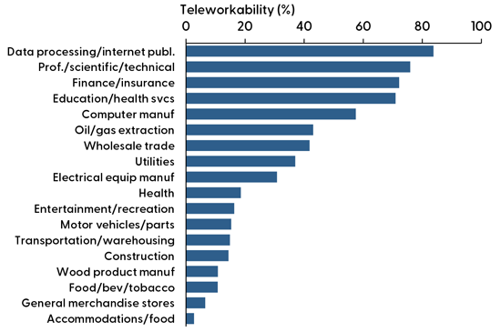
Industry productivity and teleworkability
Since industries differ considerably in their adaptability to remote work, one would imagine that the shift to telework during the pandemic would affect industries differently. For example, if teleworking offered an important way to circumvent production disruptions brought on by the pandemic, teleworkable industries would have performed better because they faced lower costs to adopting teleworking.
We next examine this relationship between teleworkability and industry productivity growth during and following the pandemic, shown in Figure 2. The horizontal axis measures teleworkability by industry, constructed from the Dingel and Neiman measures in Figure 1. The vertical axis is annualized quarterly productivity growth from the fourth quarter of 2019 to the first quarter of 2023, measured in percentage points. The size of the bubbles conveys the pre-pandemic share of an industry’s contribution to total output, measured as industry value-added, as of the fourth quarter of 2019.
Figure 2 Industry productivity growth versus teleworkability
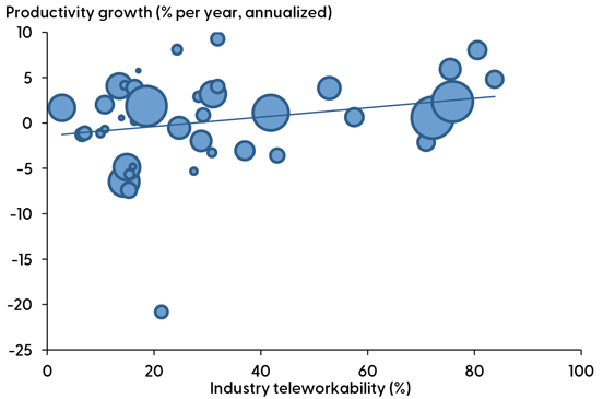
The blue fitted line reflects the average relationship between the two variables. The figure shows that more-teleworkable industries grew somewhat faster during the pandemic than less-teleworkable industries. A 1 percentage point increase in teleworkability is associated with a 0.05 percentage point increase in an industry’s predicted pandemic productivity growth rate. The relationship is statistically significant.
However, it turns out that more-teleworkable industries also grew faster before the pandemic. To better isolate the association with the shift to remote work during the pandemic, Figure 3 controls for pre-pandemic trends by removing each industry’s average annualized productivity growth for 2006–2019 from its pandemic average. Hence, the vertical axis now captures the amount by which an industry’s pandemic productivity growth exceeded or fell short of its pre-pandemic pace.
In Figure 3, the nearly flat blue line reflects that there is essentially no relationship between teleworkability and excess pandemic productivity growth. Although the association is still slightly positive, the relationship is much weaker than in Figure 2 and is not statistically significant.
Figure 3 Productivity growth, accounting for pre-pandemic trends
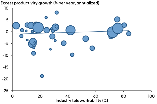
Both Figures 2 and 3, show that productivity growth varied significantly across industries. But based on Figure 3, it appears unlikely that the differences in performance during the pandemic across industries have much to do with differences in teleworking. Fernald and Li (2022) take the analysis one step further by considering that growth in work hours might be mismeasured to the extent that people are working more “off the clock” (Barrero et al. 2021). That analysis reinforces the conclusion from Figure 3, that there is essentially no relationship between teleworkability and pandemic productivity growth. We found similar results using only data during 2020 when firms were first adjusting to new work arrangements. The results are also similar for 2021-23, when firms had more experience with remote work and were also shifting to reopening office workspaces and, increasingly, to hybrid work.
The shift to remote and hybrid work has reshaped society in important ways, and these effects are likely to continue to evolve. For example, with less time spent commuting, some people have moved out of cities, and the lines between work and home life have blurred. Despite these noteworthy effects, in this Letter we find little evidence in industry data that the shift to remote and hybrid work has either substantially held back or boosted the rate of productivity growth.
Our findings do not rule out possible future changes in productivity growth from the spread of remote work. The economic environment has changed in many ways during and since the pandemic, which could have masked the longer-run effects of teleworking. Continuous innovation is the key to sustained productivity growth. Working remotely could foster innovation through a reduction in communication costs and improved talent allocation across geographic areas. However, working off-site could also hamper innovation by reducing in-person office interactions that foster idea generation and diffusion. The future of work is likely to be a hybrid format that balances the benefits and limitations of remote work.
Barrero, Jose Maria, Nicolas Bloom, and Steven J. Davis. 2021. “Why Working from Home Will Stick.” National Bureau of Economic Research Working Paper 28731. Updated survey results available from https://wfhresearch.com/ .
Bick, Alexander, Adam Blandin, and Karel Mertens. 2020. “ Work from Home before and after the COVID-19 Outbreak .” American Economic Journal: Macroeconomics 15(4), pp. 1-39.
Bloom, Nicholas, James Liang, John Roberts, and Zhichun Jenny Ying. 2015. “Does Working from Home Work? Evidence from a Chinese Experiment.” Quarterly Journal of Economics 130(1), pp. 165¬-218.
Dingel, Jonathan I., and Brent Neiman. 2020. “How Many Jobs Can Be Done at Home?” Journal of Public Economics 189(104235).
Emanuel, Natalia, and Emma Harrington. 2023. “ Working Remotely? Selection, Treatment, and the Market for Remote Work .” FRB New York Staff Report 1061 (May).
Fernald, John, and Huiyu Li. 2022. “ The Impact of COVID on Productivity and Potential Output .” Paper presented at the Federal Reserve Bank of Kansas City’s Economic Policy Symposium, Jackson Hole, WY, August 25.
Opinions expressed in FRBSF Economic Letter do not necessarily reflect the views of the management of the Federal Reserve Bank of San Francisco or of the Board of Governors of the Federal Reserve System. This publication is edited by Anita Todd and Karen Barnes. Permission to reprint portions of articles or whole articles must be obtained in writing. Please send editorial comments and requests for reprint permission to [email protected]
Along with Stanford news and stories, show me:
- Student information
- Faculty/Staff information
We want to provide announcements, events, leadership messages and resources that are relevant to you. Your selection is stored in a browser cookie which you can remove at any time using “Clear all personalization” below.
- Research led by Nicholas Bloom shows that employees who work from home for two days a week are just as productive and as likely to be promoted as their fully office-based peers.
- The study found that hybrid work had zero effect on workers’ productivity or career advancement and dramatically boosted retention rates.
It is one of the most hotly debated topics in today’s workplace: Is allowing employees to log in from home a few days a week good for their productivity, careers, and job satisfaction?
Nicholas Bloom, a Stanford economist and one of the foremost researchers on work-from-home policies, has uncovered compelling evidence that hybrid schedules are a boon to both employees and their bosses.
In a study, newly published in the journal Nature , of an experiment on more than 1,600 workers at Trip.com – a Chinese company that is one of the world’s largest online travel agencies – Bloom finds that employees who work from home for two days a week are just as productive and as likely to be promoted as their fully office-based peers.
On a third key measure, employee turnover, the results were also encouraging. Resignations fell by 33% among workers who shifted from working full-time in the office to a hybrid schedule. Women, non-managers, and employees with long commutes were the least likely to quit their jobs when their treks to the office were cut to three days a week. Trip.com estimates that reduced attrition saved the company millions of dollars.
“The results are clear: Hybrid work is a win-win-win for employee productivity, performance, and retention,” says Bloom, who is the William D. Eberle Professor of Economics at the Stanford School of Humanities and Sciences and also a senior fellow at the Stanford Institute for Economic Policy Research (SIEPR).
The findings are especially significant given that, by Bloom’s count, about 100 million workers worldwide now spend a mix of days at home and in the office each week, more than four years after COVID-19 pandemic lockdowns upended how and where people do their jobs. Many of these hybrid workers are lawyers, accountants, marketers, software engineers, and others with a college degree or higher.
Over time, though, working outside the office has come under attack from high-profile business leaders like Elon Musk, the head of Tesla, SpaceX, and X (formerly Twitter), and Jamie Dimon, CEO of JPMorgan Chase, who argue that the costs of remote work outweigh any benefits. Opponents say that employee training and mentoring, innovation, and company culture suffer when workers are not on-site five days a week.
Blooms says that critics often confuse hybrid for fully remote, in part because most of the research into working from home has focused on workers who aren’t required to come into an office and on a specific type of job, like customer support or data entry. The results of these studies have been mixed, though they tend to skew negative. This suggests to Bloom that problems with fully remote work arise when it’s not managed well.
As one of the few randomized control trials to analyze hybrid arrangements – where workers are offsite two or three days a week and are in the office the rest of the time – Bloom says his findings offer important lessons for other multinationals, many of which share similarities with Trip.com.
“This study offers powerful evidence for why 80% of U.S. companies now offer some form of remote work,” Bloom says, “and for why the remaining 20% of firms that don’t are likely paying a price.”
The research is also the largest to date of hybrid work involving university-trained professionals that rely on the gold standard in research, the randomized controlled trial. This allowed Bloom and his co-authors to show that the benefits they identified resulted from Trip.com’s hybrid experiment and not something else.
In addition to Bloom, the study’s authors are Ruobing Han, an assistant professor at The Chinese University of Hong Kong, and James Liang, an economics professor at Peking University and co-founder of Trip.com. Han and Liang both earned their PhDs in economics from Stanford.
The hybrid approach: Only winners
Trip.com didn’t have a hybrid work policy when it undertook the six-month experiment starting in 2021 that is at the heart of the study. In all, 395 managers and 1,217 non-managers with undergraduate degrees – all of whom worked in engineering, marketing, accounting, and finance in the company’s Shanghai office – participated. Employees whose birthdays fell on an even-numbered day of the month were told to come to the office five days a week. Workers with odd-numbered birthdays were allowed to work from home two days a week.
Of the study participants, 32% also had postgraduate degrees, mostly in computer science, accounting, or finance. Most were in their mid-30s, half had children, and 65% were male.
In finding that hybrid work not only helps employees, but also companies, the researchers relied on various company data and worker surveys, including performance reviews and promotions for up to two years after the experiment. Trip.com’s thorough performance review process includes evaluations of an employee’s contributions to innovation, leadership, and mentoring.
The study authors also compared the quality and amount of computer code written by Trip.com software engineers who were hybrid against code produced by peers who were in the office full-time.
In finding that hybrid work had zero effect on workers’ productivity or career advancement and dramatically boosted retention rates, the study authors highlight some important nuances. Resignations, for example, fell only among non-managers; managers were just as likely to quit whether they were hybrid or not.
Bloom and his co-authors identify misconceptions held by workers and their bosses. Workers, especially women, were reluctant to sign up as volunteers for Trip.com’s hybrid trial – likely for fear that they would be judged negatively for not coming into the office five days a week, Bloom says. In addition, managers predicted on average that remote working would hurt productivity, only to change their minds by the time the experiment ended.
For business leaders, Bloom says the study confirms that concerns that hybrid work does more harm than good are overblown.
“If managed right, letting employees work from home two or three days a week still gets you the level of mentoring, culture-building, and innovation that you want,” Bloom says. “From an economic policymaking standpoint, hybrid work is one of the few instances where there aren’t major trade-offs with clear winners and clear losers. There are almost only winners.”
Trip.com was sold: It now allows hybrid work companywide.
More From Forbes
Working from home leads to decreased productivity, research suggests.
- Share to Facebook
- Share to Twitter
- Share to Linkedin
A study shows a 10%-20% productivity decrease in remote work, sparking discussions on work models ... [+] and the need for leaders to balance efficiency and employee wellness.
The global pandemic has led to unprecedented shifts in work dynamics, with a massive transition to remote work. That said, a new study now stirs the waters of the ongoing debate about the efficiency and effectiveness of working from home, reported Fortune .
WFH Research’s latest working paper , conducted by Stanford’s Institute for Economic Policy and Research, delves deep into the question that has been looming over businesses and employees: Does working from home cause diminished productivity? The results of the study, pointing to a 10%-20% decrease in productivity for fully remote workers, have brought forth complex implications for employers, employees, and policymakers.
These findings, which are not peer reviewed , could be nothing short of a bombshell in the remote work discourse, especially among the advocates of remote work. Many firms that were on the verge of embracing a permanent remote work model may now be forced to reevaluate their stance. The implications go beyond mere statistics, opening up discussions about the quality of work, employee engagement, and the sustainability of remote work in the long term. The renewed debate may influence not only organizational policies but also broader economic and societal perspectives on remote work.
The Challenges of Remote Work
The paper—essentially a meta review of research papers undertaken to date—digs into the factors behind the drop in productivity. Top among these is less efficient communication. Remote work deprives employees of the subtle non-verbal cues and spontaneous interactions that often lead to more effective collaboration and innovation in a physical workspace. Added to this is a lack of motivation for some when working remotely. Without the communal environment of an office, some individuals may find it difficult to maintain enthusiasm and focus on tasks.
The absence of face-to-face interactions also affects mentorship and networking opportunities. Building professional relationships and learning from colleagues becomes more challenging when interactions are limited to scheduled virtual meetings. Furthermore, the blurred lines between work and home life present a significant challenge. Many employees struggle to switch off from work, leading to increased stress and potentially affecting overall well-being.
Best High-Yield Savings Accounts Of 2024
Best 5% interest savings accounts of 2024, implications for leaders.
Leaders across various industries are faced with a critical task: How to integrate these findings into their organizational strategies. It’s not just about immediate changes but about redefining the entire work model. Some businesses may see this as a sign to revert to in-person work, but that may not be the only solution.
Leaders have the opportunity to be innovative in crafting work models that combine the benefits of remote and in-person work. Creating an environment that fosters both productivity and well-being might mean reshaping office layouts, reconsidering work schedules, and innovating communication strategies. Cultural aspects, such as promoting inclusivity and maintaining engagement among remote workers, must also be addressed.
The task is immense but not insurmountable. Leaders may need to foster collaborative discussions, gather insights from employees, and be willing to experiment with various models to find what works best for their unique organizational needs.
The findings of the study do not necessarily mark the end of remote work. Instead, they may lead to a more balanced approach. Hybrid work models, combining in-person and remote work, may emerge as a preferable solution. These models can provide the flexibility that many employees value while still maintaining the community and collaboration that offices offer. Companies may need to invest in better remote working tools and training to overcome the identified challenges.
Clear policies on work hours and expectations can help in maintaining a work-life balance. The productivity dip should not overshadow the potential advantages of remote work, such as reduced commuting time, broader talent pools, and individual flexibility. A balanced approach can maximize these benefits while mitigating the challenges.
Looking Forward
The transition from traditional office work to remote or hybrid models is a complex journey filled with both opportunities and pitfalls. The study adds a significant dimension to the understanding of this transition, providing data and insights that can guide future decisions. This is far from the last word on remote work. The debate is likely to continue, fueled by further research, evolving technologies, and changing societal norms. The lessons learned will continue to shape not just the future of individual businesses but the broader landscape of work, possibly leading to a more flexible, responsive, and humane work environment.
And so, the findings of this study offer a nuanced view of the remote work scenario, emphasizing the need for deliberate, strategic, and empathetic leadership. The challenge now lies in leveraging these insights to create work environments that resonate with the new realities while nurturing both productivity and human connection.
Correction: A previous version of this story referred to the working paper as a study. This has been corrected as of August 9, 2023.

- Editorial Standards
- Reprints & Permissions
Join The Conversation
One Community. Many Voices. Create a free account to share your thoughts.
Forbes Community Guidelines
Our community is about connecting people through open and thoughtful conversations. We want our readers to share their views and exchange ideas and facts in a safe space.
In order to do so, please follow the posting rules in our site's Terms of Service. We've summarized some of those key rules below. Simply put, keep it civil.
Your post will be rejected if we notice that it seems to contain:
- False or intentionally out-of-context or misleading information
- Insults, profanity, incoherent, obscene or inflammatory language or threats of any kind
- Attacks on the identity of other commenters or the article's author
- Content that otherwise violates our site's terms.
User accounts will be blocked if we notice or believe that users are engaged in:
- Continuous attempts to re-post comments that have been previously moderated/rejected
- Racist, sexist, homophobic or other discriminatory comments
- Attempts or tactics that put the site security at risk
- Actions that otherwise violate our site's terms.
So, how can you be a power user?
- Stay on topic and share your insights
- Feel free to be clear and thoughtful to get your point across
- ‘Like’ or ‘Dislike’ to show your point of view.
- Protect your community.
- Use the report tool to alert us when someone breaks the rules.
Thanks for reading our community guidelines. Please read the full list of posting rules found in our site's Terms of Service.

An official website of the United States government
The .gov means it’s official. Federal government websites often end in .gov or .mil. Before sharing sensitive information, make sure you’re on a federal government site.
The site is secure. The https:// ensures that you are connecting to the official website and that any information you provide is encrypted and transmitted securely.
- Publications
- Account settings
Preview improvements coming to the PMC website in October 2024. Learn More or Try it out now .
- Advanced Search
- Journal List
- J Grad Med Educ
- v.8(1); 2016 Feb
Getting More Done: Strategies to Increase Scholarly Productivity
Scholarship is required for promotion at many academic institutions, and academic physicians have a multitude of competing demands on their time. This article reviews strategies for organizing time, focusing on scholarly tasks, increasing scholarly productivity, and avoiding distractions.
The “To-Do” List
Most successful people plan what they need to accomplish. It has been demonstrated that having a written plan of action increases productivity. 1 , 2 Studies looking at the effect of writing down a list of things to do date back to the 1920s and an Eastern European psychologist named Bluma Zeigarnik. The so-called “Zeigarnik Effect” demonstrated that the act of planning activities through “to-do” lists actually reduced executive burden on the brain by freeing the brain from having to worry about unfinished tasks. 1 More recent studies confirmed the Zeigarnik Effect by finding that when people were not allowed to finish a warm-up activity, they performed poorly on a subsequent brainstorming activity. 2 The implication is that people are more effective when they are able to cross off the first thing on their list. It allows them to go on to the next thing.
There are multiple ways to keep track of things to do. The traditional to-do list is created with a pen and paper. There are also multiple electronic to-do list applications for computers, tablets, or smartphones. 3 Stephen Covey, in The 7 Habits of Highly Effective People , 4 describes a method of setting goals and then prioritizing tasks within those goals. He recommends prioritizing to-do lists into urgent and not urgent, important and not important. For faculty who are writing scholarly papers, breaking down each task into smaller tasks will help make the to-do list more effective. For instance, instead of putting “write paper” on the list, you can itemize each individual component, such as “write introduction” or “make tables.”
Finding a Balance: Learning to Say “No”
Once your to-do list is organized, it is time to focus on the actual tasks you need to do. Since each day has a limited number of hours, it makes sense to spend these hours on important tasks. Using time wisely includes limiting your workload to activities that are directly related to career goals. In doing this, you may be required to say “no” to certain requests for your time.
Saying “no” can be difficult for several reasons. The first reason is the inherent desire to help out colleagues if possible, so the first inclination is to say “yes” to a new request for help. However, saying “yes” to a project, committee, or work group that is not interesting or not aligned with career goals will potentially not allow enough time to complete work that is in your area of interest. Second, being a team player is important and saying “no” may be thought of as selfish, or may jeopardize a relationship ( table 1 ). Finding the right balance between aiding colleagues by saying “yes” to some requests, while also protecting time for your own work, can be challenging.
Saying “Yes” and “No”

There are several ways to say “no.” 5 Most time management experts recommend never saying “yes” or “no” on the spot. 6 It takes practice, but is ultimately very helpful to always say something like, “Thank you so much for asking me. I'm going to look at my other work and see whether I think I can give this project/committee/work group enough time to do a good job.” Another option for junior faculty is to consult their mentors before saying “yes” to a request. Obviously, if a request is exciting and closely related to your area of interest, saying “yes” seems obvious, but consider the request first. Can you negotiate to get something else off your plate so that you have adequate time for the new project? Can you negotiate for administrative support or time away from clinical duties? Even if what you want your answer to be is obvious to you, spend a day or two thinking about it. The trick is to have a clear idea in your head of what you love to do, what you like to do, and what you are required to do. Then, saying “yes” and “no” can be based on that, in conjunction with work responsibilities ( box ).
box How to Decide Whether to Say “Yes” or “No”
- Does the request fit with your career goals?
- Would the work use your skills?
- What is the long-term benefit of this work? Could it lead to other work that is more closely related to your goals?
- What is the timing of this work? Does it need to be done within a week, a month, or can it be done more long term when you may have more time?
- Can you be involved in part of the work but not all?
- Are you able to give up another responsibility in order to take on the new request?
- Is the requestor someone who is your supervisor or who can influence your career?
- Would saying “no” jeopardize other parts of your job or career goals?
Increasing Productivity by Making Everything Count Twice
Faculty can demonstrate a scholarly approach to patient care and teaching by developing scholarly products based on clinical or educational work. For example, if you enjoy taking care of patients with a specific disease (X), you may collect patient cases and focus your educational material on the presentation, management, and follow-up of patients with disease X. Making your clinical interests into scholarly products may involve using the lectures you have put together on disease X and writing a review article for a specialty journal. You may also involve trainees in developing posters and presentations on different aspects of disease X to present at meetings ( table 2 ).
Making Everything Count Twice: The Art of Using Day-to-Day Work as Scholarship

Being Efficient
To be more productive, we need to focus. Multitasking is a misnomer because our brains can really only focus on 1 task at a time. When we think we are doing 3 things at once, our brains actually switch back and forth from task to task. In a 2006 study that used functional magnetic resonance imaging to document the activation of different parts of people's brains as they went from one activity to another, only 1 area was activated at a time. The researchers also documented what they called a “bottleneck” at a central area of information processing, which allowed only 1 thought through at a time. 11 Other research has shown that it takes 30 to 60 seconds to refocus on 1 task after transferring attention to a second one. The more complex the task (ie, analyzing data or writing an abstract) the longer it takes to refocus. It has been estimated that multitasking can reduce productivity up to 40% and actually decrease intelligence quotients up to 10 points. 12
Finding a time to write a paper is challenging when clinical or other standing duties are ever-present. We all struggle with issues or habits that distract us and make us less productive. 13 , 14 It is important to identify the specific causes of procrastination and learn techniques to minimize time spent on unimportant tasks that distract us from pursuing our scholarly work ( table 3 ). Some successful academic physicians designate time each week as writing time, to limit the number of clinical phone calls and interruptions that they receive. 8 Faculty members who write regularly are more productive than those who “binge write.” 15 Furthermore, avoiding interruptions of academic work by e-mail, Internet searches, or text messages will lead to more focused academic time and increased scholarly productivity. 9
Common Distractions and Techniques to Minimize Them

Academic faculty are very busy, and often wish for more hours in the day. Developing a plan of action, learning to be efficient, and limiting requests for time that do not align with personal career goals should help faculty members accomplish more in the same amount of time while boosting scholarly productivity.
Both authors are at the University of Wisconsin, Madison. Sarina Schrager, MD, MS, is Professor, Department of Family Medicine; and Elizabeth Sadowski, MD, is Associate Professor, Departments of Radiology and Obstetrics and Gynecology.
Americans are embracing flexible work—and they want more of it
Get the latest.
July 10, 2024
In the time since we first published this article, McKinsey has continued to explore the topic. Read on for a summary of our latest insights.
“How often do you go into the office?” Today, this question typifies the postpandemic era, just as the phrases “social distancing” and “PCR test” did in 2020. The answer? Probably more than you did during those early days of reentry after the pandemic’s peak, but probably less than you did in 2019.
Our research shows that hybrid work is here to stay . Office attendance remains roughly 30 percent lower than it was before the pandemic. Attendance is especially low in metropolitan areas like London, New York, and San Francisco with large shares of knowledge-economy workers and expensive housing. In these markets, when employees do go into the office, the primary reason is to connect with their teams.
But can remote work be productive work? That depends on whom you ask. Eighty-three percent of employees we surveyed cite the ability to work more efficiently and productively as a primary benefit of working remotely. Our research indicates that even fully remote companies with the right operating models can outperform their in-person peers on organizational health. But many companies see this quite differently : only half of HR leaders say employee productivity is a primary benefit of working remotely.
According to Nicholas Bloom, the William Eberle Professor of Economics at Stanford University and a senior fellow at the Stanford Institute for Economic Policy Research, there is a productivity benefit from what he calls “ well-organized hybrid ” work environments. In this scenario, everybody comes into the office on the same days, allowing employees to maximize their time together. When you factor in the time saved from not having to commute, as well as the benefit of working in a quieter and more controlled home environment, the result, says Bloom, is a productivity improvement of up to 5 percent . (Of course, some homes are quieter and more controlled than others.)
Who values workplace flexibility the most? The majority of employees say that the opportunity to work remotely is a top company benefit. Both women and men cite less fatigue and burnout as a benefit of hybrid and remote work. But women, particularly those with childcare duties, continue to prize it more. In fact, 38 percent of mothers with young children say that without workplace flexibility they would have had to reduce their work hours or leave their companies.
Many organizations are still trying to find the right balance as they attempt to create true hybrid work models. This may be because they are hesitant to expend the financial and leadership resources necessary to create magnetic and inclusive work environments. But the potential upsides—including real estate savings, a more diverse and inclusive workforce, and improved employee satisfaction and performance—may be well worth the effort .
Articles referenced include:
- Women in the Workplace 2023 , October 2023
- How hybrid work has changed the way people work, live, and shop , July 2023
- Is your workplace ready for flexible work? A survey offers clues , June 2023
- Forward Thinking on how to get remote working right with Nicholas Bloom , February 2023
When the COVID-19 pandemic shuttered workplaces nationwide, society was plunged into an unplanned experiment in work from home. Nearly two-and-a-half years on, organizations worldwide have created new working norms that acknowledge that flexible work is no longer a temporary pandemic response but an enduring feature of the modern working world.
About the survey
This article is based on a 25-minute, online-only Ipsos poll conducted on behalf of McKinsey between March 15 and April 18, 2022. A sample of 25,062 adults aged 18 and older from the continental United States, Alaska, and Hawaii was interviewed online in English and Spanish. To better reflect the population of the United States as a whole, post hoc weights were made to the population characteristics on gender, age, race/ethnicity, education, region, and metropolitan status. Given the limitations of online surveys, 1 “Internet surveys,” Pew Research Center. it is possible that biases were introduced because of undercoverage or nonresponse. People with lower incomes, less education, people living in rural areas, or people aged 65 and older are underrepresented among internet users and those with high-speed internet access.
The third edition of McKinsey’s American Opportunity Survey provides us with data on how flexible work fits into the lives of a representative cross section of workers in the United States. McKinsey worked alongside the market-research firm Ipsos to query 25,000 Americans in spring 2022 (see sidebar, “About the survey”).
The most striking figure to emerge from this research is 58 percent. That’s the number of Americans who reported having the opportunity to work from home at least one day a week. 1 Many of the survey questions asked respondents about their ability or desire to “work from home.” “Work from home” is sometimes called “remote work,” while arrangements that allow for both remote and in-office work are often interchangeably labeled “hybrid” or “flexible” arrangements. We prefer the term flexible, which acknowledges that home is only one of the places where work can be accomplished and because it encompasses a variety of arrangements, whereas hybrid implies an even split between office and remote work. Thirty-five percent of respondents report having the option to work from home five days a week. What makes these numbers particularly notable is that respondents work in all kinds of jobs, in every part of the country and sector of the economy, including traditionally labeled “blue collar” jobs that might be expected to demand on-site labor as well as “white collar” professions.
About the authors
This article is a collaborative effort by André Dua , Kweilin Ellingrud , Phil Kirschner , Adrian Kwok, Ryan Luby, Rob Palter , and Sarah Pemberton as part of ongoing McKinsey research to understand the perceptions of and barriers to economic opportunity in America. The following represents the perspectives of McKinsey’s Real Estate and People & Organizational Performance Practices.
Another of the survey’s revelations: when people have the chance to work flexibly, 87 percent of them take it. This dynamic is widespread across demographics, occupations, and geographies. The flexible working world was born of a frenzied reaction to a sudden crisis but has remained as a desirable job feature for millions. This represents a tectonic shift in where, when, and how Americans want to work and are working.
The following six charts examine the following:
- the number of people offered flexible working arrangements either part- or full-time
- how many days a week employed people are offered and do work from home
- the gender, age, ethnicity, education level, and income of people working or desiring to work flexibly
- which occupations have the greatest number of remote workers and how many days a week they work remotely
- how highly employees rank flexible working arrangements as a reason to seek a new job
- impediments to working effectively for people who work remotely all the time, part of the time, or not at all
Flexible work’s implications for employees and employers—as well as for real estate, transit, and technology, to name a few sectors—are vast and nuanced and demand contemplation.
1. Thirty-five percent of job holders can work from home full-time, and 23 percent can do so part-time
A remarkable 58 percent of employed respondents—which, extrapolated from the representative sample, is equivalent to 92 million people from a cross section of jobs and employment types—report having the option to work from home for all or part of the week. After more than two years of observing remote work and predicting that flexible working would endure after the acute phases of the COVID-19 pandemic, we view these data as a confirmation that there has been a major shift in the working world and in society itself.
We did not ask about flexible work in our American Opportunity Survey in past years, but an array of other studies indicate that flexible working has grown by anywhere from a third to tenfold since 2019. 1 Rachel Minkin et al., “How the coronavirus outbreak has—and hasn’t—changed the way Americans work,” Pew Research Center, December 9, 2020; “Telework during the COVID-19 pandemic: Estimates using the 2021 Business Response Survey,” US Bureau of Labor Statistics, Monthly Labor Review, March 2022.
Thirty-five percent of respondents say they can work from home full-time. Another 23 percent can work from home from one to four days a week. A mere 13 percent of employed respondents say they could work remotely at least some of the time but opt not to.
Forty-one percent of employed respondents don’t have the choice. This may be because not all work can be done remotely or because employers simply demand on-site work. Given workers’ desire for flexibility, employers may have to explore ways to offer the flexibility employees want to compete for talent effectively.
2. When offered, almost everyone takes the opportunity to work flexibly
The results of the survey showed that not only is flexible work popular, with 80 million Americans engaging in it (when the survey results are extrapolated to the wider population), but many want to work remotely for much of the week when given the choice.
Eighty-seven percent of workers offered at least some remote work embrace the opportunity and spend an average of three days a week working from home. People offered full-time flexible work spent a bit more time working remotely, on average, at 3.3 days a week. Interestingly, 12 percent of respondents whose employers only offer part-time or occasional remote work say that even they worked from home for five days a week. This contradiction appears indicative of a tension between how much flexibility employers offer and what employees demand .
3. Most employees want flexibility, but the averages hide the critical differences
There’s remarkable consistency among people of different genders, ethnicities, ages, and educational and income levels: the vast majority of those who can work from home do so. In fact, they just want more flexibility: although 58 percent of employed respondents say they can work from home at least part of the time, 65 percent of employed respondents say they would be willing to do so all the time.
However, the opportunity is not uniform: there was a large difference in the number of employed men who say they were offered remote-working opportunities (61 percent) and women (52 percent). At every income level, younger workers were more likely than older workers to report having work-from-home opportunities.
People who could but don’t work flexibly tend to be older (19 percent of 55- to 64-year-olds offered remote work didn’t take it, compared with 12 to 13 percent of younger workers) or have lower incomes (17 percent of those earning $25,000 to $74,999 per year who were offered remote work didn’t take it, compared with 10 percent of those earning over $75,000 a year). While some workers may choose to work on-site because they prefer the environment, others may feel compelled to because their home environments are not suitable, because they lack the skills and tools to work remotely productively, or because they believe there is an advantage to being on-site. Employers should be aware that different groups perceive and experience remote work differently and consider how flexible working fits with their diversity, equity, and inclusion strategies .
4. Most industries support some flexibility, but digital innovators demand it
The opportunity to work flexibly differs by industry and role within industries and has implications for companies competing for talent. For example, the vast majority of employed people in computer and mathematical occupations report having remote-work options, and 77 percent report being willing to work fully remotely. Because of rapid digital transformations across industries , even those with lower overall work-from-home patterns may find that the technologists they employ demand it.
A surprisingly broad array of professions offer remote-work arrangements. Half of respondents working in educational instruction and library occupations and 45 percent of healthcare practitioners and workers in technical occupations say they do some remote work, perhaps reflecting the rise of online education and telemedicine. Even food preparation and transportation professionals said they do some work from home.
5. Job seekers highly value having autonomy over where and when they work
The survey asked people if they had hunted for a job recently or were planning to hunt for one. Unsurprisingly, the most common rationale for a job hunt was a desire for greater pay or more hours, followed by a search for better career opportunities. The third-most-popular reason was looking for a flexible working arrangement.
Prior McKinsey research has shown that for those that left the workforce during the early phases of the COVID-19 pandemic, workplace flexibility was a top reason that they accepted new jobs . Employers should be aware that when a candidate is deciding between job offers with similar compensation, the opportunity to work flexibly can become the deciding factor.
6. Employees working flexibly report obstacles to peak performance
The survey asked respondents to identify what made it hard to perform their jobs effectively. Those working in a flexible model were most likely to report multiple obstacles, followed by those working fully remotely, and then by those working in the office. Our research doesn’t illuminate the cause and effect here: it could be that people who face barriers are more likely to spend some time working from home. It could also be that workers who experience both on-site and at-home work are exposed to the challenges of each and the costs of regularly switching contexts.
Some obstacles were reported at much higher rates by specific groups: for example, about 55 percent of 18- to 34-year-olds offered the option to work fully remotely say mental-health issues impacted their ability to perform effectively, though only 17 percent of people aged 55 to 64 said the same. Workers with children at home who were offered full-time remote-work options were far more likely than their peers without children to report that problems with physical health or a hostile work environment had a moderate or major impact on their job.
The results of the American Opportunity Survey reflect sweeping changes in the US workforce, including the equivalent of 92 million workers offered flexible work, 80 million workers engaged in flexible work, and a large number of respondents citing a search for flexible work as a major motivator to find a new job.
Competition for top performers and digital innovators demands that employers understand how much flexibility their talent pool is accustomed to and expects. Employers are wise to invest in technology, adapt policies, and train employees to create workplaces that integrate people working remotely and on-site (without overcompensating by requiring that workers spend too much time in video meetings ). The survey results identify obstacles to optimal performance that underscore a need for employers to support workers with issues that interfere with effective work. Companies will want to be thoughtful about which roles can be done partly or fully remotely—and be open to the idea that there could be more of these than is immediately apparent. Employers can define the right metrics and track them to make sure the new flexible model is working.
At a more macro level, a world in which millions of people no longer routinely commute has meaningful implications for the commercial core in big urban centers and for commercial real estate overall. Likewise, such a world implies a different calculus for where Americans will live and what types of homes they will occupy. As technology emerges that eliminates the residual barriers to more distributed and asynchronous work, it could become possible to move more types of jobs overseas, with potentially significant consequences.
In time, the full impact of flexible working will be revealed. Meanwhile, these data give us early insight into how the working world is evolving.
For more on the imperative for flexible work and how organizations can respond, please see McKinsey.com/featured-insights/ Future-of-the-workplace .
André Dua is a senior partner in McKinsey’s Miami office; Kweilin Ellingrud is a senior partner in the Minneapolis office; Phil Kirschner is a senior expert in the New York office, where Adrian Kwok is an associate partner and Ryan Luby is a senior expert; Rob Palter is a senior partner in the Toronto office; and Sarah Pemberton is a manager in the Hong Kong office.
Explore a career with us
Related articles.

Hybrid work: Making it fit with your diversity, equity, and inclusion strategy

Workplace real estate in the COVID-19 era: From cost center to competitive advantage
Multitasking: Switching costs
What the research shows.
Doing more than one task at a time, especially more than one complex task, takes a toll on productivity. Although that shouldn't surprise anyone who has talked on the phone while checking E-mail or talked on a cell phone while driving, the extent of the problem might come as a shock. Psychologists who study what happens to cognition (mental processes) when people try to perform more than one task at a time have found that the mind and brain were not designed for heavy-duty multitasking. Psychologists tend to liken the job to choreography or air-traffic control, noting that in these operations, as in others, mental overload can result in catastrophe.
Multitasking can take place when someone tries to perform two tasks simultaneously, switch . from one task to another, or perform two or more tasks in rapid succession. To determine the costs of this kind of mental "juggling," psychologists conduct task-switching experiments. By comparing how long it takes for people to get everything done, the psychologists can measure the cost in time for switching tasks. They also assess how different aspects of the tasks, such as complexity or familiarity, affect any extra time cost of switching.
In the mid-1990s, Robert Rogers, PhD, and Stephen Monsell, D.Phil, found that even when people had to switch completely predictably between two tasks every two or four trials, they were still slower on task-switch than on task-repeat trials. Moreover, increasing the time available between trials for preparation reduced but did not eliminate the cost of switching. There thus appear to be two parts to the switch cost -- one attributable to the time taken to adjust the mental control settings (which can be done in advance it there is time), and another part due to competition due to carry-over of the control settings from the previous trial (apparently immune to preparation).
Surprisingly, it can be harder to switch to the more habitual of two tasks afforded by a stimulus. For example, Renata Meuter, PhD, and Alan Allport, PhD, reported in 1999 that if people had to name digits in their first or second language, depending on the color of the background, as one might expect they named digits in their second language slower than in their first when the language repeated. But they were slower in their first language when the language changed.
In experiments published in 2001, Joshua Rubinstein, PhD, Jeffrey Evans, PhD, and David Meyer, PhD, conducted four experiments in which young adults switched between different tasks, such as solving math problems or classifying geometric objects. For all tasks, the participants lost time when they had to switch from one task to another. As tasks got more complex, participants lost more time. As a result, people took significantly longer to switch between more complex tasks. Time costs were also greater when the participants switched to tasks that were relatively unfamiliar. They got up to speed faster when they switched to tasks they knew better.
In a 2003 paper, Nick Yeung, Ph.D, and Monsell quantitatively modeled the complex and sometimes surprising experimental interactions between relative task dominance and task switching. The results revealed just some of the complexities involved in understanding the cognitive load imposed by real-life multi-tasking, when in addition to reconfiguring control settings for a new task, there is often the need to remember where you got to in the task to which you are returning and to decide which task to change to, when.
What the research means
According to Meyer, Evans and Rubinstein, converging evidence suggests that the human "executive control" processes have two distinct, complementary stages. They call one stage "goal shifting" ("I want to do this now instead of that") and the other stage "rule activation" ("I'm turning off the rules for that and turning on the rules for this"). Both of these stages help people to, without awareness, switch between tasks. That's helpful. Problems arise only when switching costs conflict with environmental demands for productivity and safety.
Although switch costs may be relatively small, sometimes just a few tenths of a second per switch, they can add up to large amounts when people switch repeatedly back and forth between tasks. Thus, multitasking may seem efficient on the surface but may actually take more time in the end and involve more error. Meyer has said that even brief mental blocks created by shifting between tasks can cost as much as 40 percent of someone's productive time.
How we use the research
Understanding the hidden costs of multitasking may help people to choose strategies that boost their efficiency - above all, by avoiding multitasking, especially with complex tasks. (Throwing in a load of laundry while talking to a friend will probably work out all right.) For example, losing just a half second of time to task switching can make a life-or-death difference for a driver on a cell phone traveling at 30 MPH. During the time the driver is not totally focused on driving the car, it can travel far enough to crash into an obstacle that might otherwise have been avoided.
Meyer and his colleagues hope that understanding switching costs and the light they shed on "executive control" may help to improve the design and engineering of equipment and human-computer interfaces for vehicle and aircraft operation, air traffic control, and many other activities using sophisticated technologies. Insights into how the brain "multitasks" lend themselves to a range of settings from the clinic, helping to diagnose and help brain-injured patients, to the halls of Congress, informing government and industrial regulations and standards.
This research is also taken into account by states and localities considering legislation to restrict drivers' use of cell phones.
Sources & further reading
Gopher, D., Armony, L. & Greenspan, Y. (2000). Switching tasks and attention policies. Journal of Experimental Psychology: General, 129 , 308-229.
Mayr, U. & Kliegl, R. (2000). Task-set switching and long-term memory retrieval. Journal of Experimental Psychology: Learning, Memory, and Cognition, 26 , 1124-1140.
Meuter, R. F. I. & Allport, A. (1999). Bilingual language switching in naming: Asymmetrical costs of language selection. Journal of Memory and Language, 40(1) , 25-40.
Meyer, D. E. & Kieras, D. E. (1997a). A computational theory of executive cognitive processes and multiple-task performance: Part 1. Basic mechanisms. Psychological Review, 104 , 3-65.
Meyer, D. E. & Kieras, D. E. (1997b). A computational theory of executive cognitive processes and multiple-task performance: Part 2. Accounts of psychological refractory-period phenomena. Psychological Review, 104 , 749-791.
Monsell, S., Azuma, R., Eimer, M., Le Pelley, M., & Strafford, S. (1998, July). Does a prepared task switch require an extra (control) process between stimulus onset and response selection? Poster presented at the 18th International Symposium on Attention and Performance, Windsor Great Park, United Kingdom.
Monsell, S., Yeung, N., & Azuma, R. (2000). Reconfiguration of task-set: Is it easier to switch to the weaker task? Psychological Research, 63 , 250-264.
Monsell, S. & Driver, J., Eds. (2000). Control of cognitive processes: Attention and Performance XVIII. Cambridge, Mass.: MIT Press.
Rogers, R. & Monsell, S. (1995). The costs of a predictable switch between simple cognitive tasks. Journal of Experimental Psychology: General, 124, 207-231.
Rubinstein, J., Evans, J. & Meyer, D. E. (1994). Task switching in patients with prefrontal cortex damage. Poster presented at the meeting of the Cognitive Neuroscience Society, San Francisco, CA, March, 1994. Abstract published in Journal of Cognitive Neuroscience , 1994, Vol. 6.
Rubinstein, J. S., Meyer, D. E. & Evans, J. E. (2001). Executive Control of Cognitive Processes in Task Switching. Journal of Experimental Psychology: Human Perception and Performance, 27 , 763-797.
Yeung, N. & Monsell, S. (2003). Switching between tasks of unequal familiarity: The role of stimulus-attribute and response-set selection. Journal of Experimental Psychology-Human Perception and Performance, 29(2) : 455-469.
The Research Is Clear: Long Hours Backfire for People and for Companies
by Sarah Green Carmichael

Managers want employees to put in long days, respond to their emails at all hours, and willingly donate their off-hours — nights, weekends, vacation — without complaining. The underlings in this equation have little control; overwork cascades from the top of the organizational pyramid to the bottom. At least, that’s one narrative of overwork. In this version, we work long hours because our bosses tell us to. (That’s the version most on display in the recent New York Times opus on Amazon .)
Partner Center
- Open access
- Published: 02 September 2024
Leadership support and satisfaction of healthcare professionals in China’s leading hospitals: a cross-sectional study
- Jinhong Zhao 1 , 2 ,
- Tingfang Liu 2 &
- Yuanli Liu 2
BMC Health Services Research volume 24 , Article number: 1016 ( 2024 ) Cite this article
Metrics details
Healthcare professionals’ job satisfaction is a critical indicator of healthcare performance, pivotal in addressing challenges such as hospital quality outcomes, patient satisfaction, and staff retention rates. Existing evidence underscores the significant influence of healthcare leadership on job satisfaction. Our study aims to assess the impact of leadership support on the satisfaction of healthcare professionals, including physicians, nurses, and administrative staff, in China’s leading hospitals.
A cross-sectional survey study was conducted on healthcare professionals in three leading hospitals in China from July to December 2021. These hospitals represent three regions in China with varying levels of social and economic development, one in the eastern region, one in the central region, and the third in the western region. Within each hospital, we employed a convenience sampling method to conduct a questionnaire survey involving 487 healthcare professionals. We assessed perceived leadership support across five dimensions: resource support, environmental support, decision support, research support, and innovation encouragement. Simultaneously, we measured satisfaction using the MSQ among healthcare professionals.
The overall satisfaction rate among surveyed healthcare professionals was 74.33%. Our study revealed significant support from senior leadership in hospitals for encouraging research (96.92%), inspiring innovation (96.30%), and fostering a positive work environment (93.63%). However, lower levels of support were perceived in decision-making (81.72%) and resource allocation (80.08%). Using binary logistic regression with satisfaction as the dependent variable and healthcare professionals’ perceived leadership support, hospital origin, job role, department, gender, age, education level, and professional designation as independent variables, the results indicated that support in resource provision (OR: 4.312, 95% CI: 2.412 ∼ 7.710) and environmental facilitation (OR: 4.052, 95% CI: 1.134 ∼ 14.471) significantly enhances healthcare personnel satisfaction.
The findings underscore the critical role of leadership support in enhancing job satisfaction among healthcare professionals. For hospital administrators and policymakers, the study highlights the need to focus on three key dimensions: providing adequate resources, creating a supportive environment, and involving healthcare professionals in decision-making processes.
Peer Review reports
Introduction
In the era of accelerated globalization, the investigation of global leadership has assumed heightened significance [ 1 ]. Leadership, as a dynamic and evolving process, holds the potential to cultivate both the personal and professional growth of followers [ 2 ]. Effective healthcare leadership can enhance medical service quality, patient safety, and staff job satisfaction through skill development, vision establishment, and clear direction-setting [ 3 , 4 , 5 ]. Moreover, leadership support can effectively enhance staff well-being and work efficiency [ 6 , 7 ]. For example, Mendes et al. found that the quality of healthcare is significantly influenced by four dimensions of leadership: communication, recognition, development, and innovation [ 8 ]. Additionally, Shanafelt et al. discovered that leaders can effectively reduce employee burnout and subsequently improve the quality of medical services by formulating and implementing targeted work interventions and motivating employees [ 9 ].
Job satisfaction among healthcare professionals is a crucial indicator of healthcare performance, playing a vital role in addressing challenges related to hospital quality outcomes, patient satisfaction, and nurse retention rates [ 10 , 11 , 12 , 13 ]. Researchers from different national backgrounds have conducted studies on the job satisfaction of healthcare workers across various disciplines. For example, Balasubramanian et al. examined the satisfaction of immigrant dentists in Australia [ 14 ], Mascari et al. studied physicians and hospital researchers in the United States [ 15 ], and Rosta et al. investigated the satisfaction of doctors in Norway [ 12 ]. Research has demonstrated that characteristics of the work environment, balanced workloads, relationships with colleagues, career opportunities, and leadership support all influence job satisfaction [ 16 ]. Several instruments are commonly used to measure job satisfaction, each relevant depending on the context and discipline. For instance, the Job Descriptive Index (JDI) focuses on different facets of job satisfaction such as work, pay, promotion, supervision, and co-workers [ 17 ]. The Job Satisfaction Survey (JSS) covers similar dimensions and is particularly useful in public sector organizations due to its comprehensive nature and ease of use [ 18 ]. The Minnesota Satisfaction Questionnaire (MSQ) is a comprehensive tool that assesses employee satisfaction across multiple dimensions including intrinsic and extrinsic satisfaction, and is commonly used for evaluating job satisfaction in the healthcare field [ 19 ].
Recent studies have linked leadership to healthcare professionals’ job satisfaction, highlighting the pivotal role of leadership in guiding, coordinating, and motivating employees [ 5 ]. For instance, the Mayo Clinic found that leadership from immediate supervisors could alleviate burnout and increase job satisfaction [ 20 ]. Choi’s research indicated that leadership empowerment significantly enhances nursing staff’s job satisfaction [ 21 ]. Additionally, Liu discovered that the support provided by hospital senior leadership is closely associated with employee satisfaction [ 22 ].
In China, while leadership research has gained some traction in areas such as business and education, it remains relatively scarce within healthcare institutions. Existing studies primarily focus on the nursing sector, and comprehensive assessments of leadership at the leading public hospitals (top 10% of Chinese hospitals) have not been extensively conducted [ 23 , 24 ]. Research on leadership and healthcare professionals’ satisfaction often relies on single indicators to measure job satisfaction, such as overall job satisfaction or specific aspects like compensation satisfaction and burnout levels [ 25 ]. This narrow focus may fail to fully capture the multidimensional nature of employee satisfaction, which includes aspects such as workload, ability utilization, sense of achievement, initiative, training and self-development, and interpersonal communication [ 26 ]. Additionally, most existing studies focus on the job satisfaction of nurses or physicians in isolation, lacking comparative research across different groups within healthcare institutions, such as doctors, nurses, and administrative personnel [ 27 , 28 , 29 ].
Therefore, this study utilized the MSQ to conduct a thorough assessment of employee satisfaction and assess the impact of leadership support on the satisfaction of healthcare personnel in China’s leading public hospitals. Through this research, we aim to enhance the core competitiveness of hospitals and provide valuable data to support leadership assessments in developing countries’ healthcare institutions. Moreover, this study seeks to contribute to the broader international understanding of effective leadership practices in China’s leading public hospitals, with implications for global health management strategies.
Study design and participants
From July to December 2021, a cross-sectional survey study was conducted on healthcare professionals in China’s 3 leading hospitals. The 3 leading hospitals represent three regions in China with different levels of social and economic development, one in the eastern, one in the central, and one in the western. In each hospital, a convenience sampling method was used to conduct a questionnaire survey among physicians, nurses, and administrative staff.
Criteria for inclusion of healthcare professionals: (1) employed at the hospital for at least 1 year or more; (2) formal employees of the hospital (full-time staff); (3) possessing cognitive clarity and the ability to independently understand and respond to electronic questionnaires, as assessed by their leaders. Exclusion criteria: (1) diagnosed with mental health disorders that impair their ability to participate, as identified by the hospital’s mental health professionals; (2) unable to communicate effectively due to severe language barriers, hearing impairments, or other communication disorders, as determined by their direct supervisors or relevant medical evaluations; (3) visiting scholars, interns, or graduate students currently enrolled in a degree program.
Instrument development
Leadership support.
In reference to the Malcolm Baldrige National Quality Award (MBNQA) framework and Supporting Relationship Theory [ 6 , 30 , 31 ], we determined the survey scale after three expert discussions involving 5–7 individuals. These experts included personnel from health administrative departments, leading public hospital leaders, middle management, and researchers specializing in hospital management. Their collective expertise ensured that the survey comprehensively assessed leadership support within hospitals from the perspective of healthcare personnel. The Leadership Support Scale consists of 5 items: Environmental Support: ‘My leaders provide a work environment that helps me perform my job,’ Resource Support: ‘My leaders provide the resources needed to improve my work,’ Decision Support: ‘My leaders support my decisions to satisfy patients,’ Research Support: ‘My leaders support my application for scientific research projects,’ and Innovation Encouragement: ‘My leaders encourage me to innovate actively and think about problems in new ways‘ (Supplementary material). All questionnaire items are rated on a 5-point Likert scale, ranging from 1 = Strongly Disagree to 5 = Strongly Agree. The Cronbach’s alpha coefficient for the 5-item scale is 0.753.
Job satisfaction
The measurement of job satisfaction was carried out using the Minnesota Satisfaction Questionnaire (MSQ) [ 32 , 33 ], which has been widely used and has been shown by scholars to have good reliability and validity in China [ 34 , 35 ]. The questionnaire consists of 20 items that measure healthcare personnel’s satisfaction with various aspects of their job, including individual job load, ability utilization, achievement, initiative, hospital training and self-development, authority, hospital policies and practices, compensation, teamwork, creativity, independence, moral standards, hospital rewards and punishments, personal responsibility, job security, social service contribution, social status, employee relations and communication, and hospital working conditions and environment. Responses to these items were balanced and rated on a scale from 1 to 5, with 1 = Very Dissatisfied, 2 = Dissatisfied, 3 = Neither Dissatisfied nor Satisfied, 4 = Satisfied, and 5 = Very Satisfied. Scores range from 20 to 100, with higher scores indicating higher satisfaction. In this study, a comprehensive assessment of healthcare personnel’s job satisfaction was made using a score of 80 and above [ 32 ], where a score of ≥ 80 was considered satisfied, and below 80 was considered dissatisfied. The Cronbach’s alpha coefficient for the questionnaire in this survey was 0.983.
Investigation process
The survey was administered through an online platform “Wenjuanxing”, and distributed by department heads to healthcare professionals within their respective departments. The selection of departments and potential participants followed a structured process: (1) Potential participants were identified based on the inclusion criteria, which were communicated to the department heads. (2) Department heads received a digital link to the survey, which they forwarded to eligible staff members via email or internal communication platforms. (3) The informed consent form was integrated into the survey link, detailing the research objectives, ensuring anonymity, and emphasizing voluntary participation. At the beginning of the online survey, participants were asked if they agreed to participate. Those who consented continued with the survey, while those who did not agree were directed to end the survey immediately.
According to Kendall’s experience and methodology, the sample size can be 5–10 times the number of independent variables (40 items) [ 36 , 37 ]. Our sample size is ten times the number of independent variables. Considering potentially disqualified questionnaires, the sample size was increased by 10%, resulting in a minimum total sample size of 460. Therefore, we distributed 500 survey questionnaires.
Data analysis
We summarized the sociodemographic characteristics of healthcare personnel survey samples using descriptive statistical methods. For all variables, we calculated the frequencies and percentages of categorical variables. Different sociodemographic characteristics in relation to healthcare personnel’s perception of leadership support and satisfaction were analyzed using the Pearson χ² test. We employed a binary logistic regression model to estimate the risk ratio of healthcare personnel satisfaction under different levels of leadership support. Estimates from three sequentially adjusted models were reported to transparently demonstrate the impact of various adjustments: (1) unadjusted; (2) adjusted for hospital of origin; (3) adjusted for hospital of origin, gender, age, education level, job type, and department. For the binary logistic regression model, we employed a backward stepwise regression approach, with inclusion at P < 0.05 and exclusion at P > 0.10 criteria. In all analyses, a two-tailed p -value of < 0.05 was considered significant, and all analyses were conducted using SPSS 26.0 (IBM Corp., Armonk, NY, USA).
Demographic characteristics and job satisfaction
This study recruited a total of 500 healthcare personnel from hospitals to participate in the survey, with 487 valid questionnaires collected, resulting in an effective response rate of 97.4%. The majority of participants were female (77.21%), with ages concentrated between 30 and 49 years old (73.71%). The predominant job titles were mid-level (45.17%) and junior-level (27.31%), and educational backgrounds were mostly at the undergraduate (45.17%) and graduate (48.25%) levels. The marital status of most participants was married (79.88%), and their primary departments were surgery (38.19%) and internal medicine (24.85%). The overall satisfaction rate among the sampled healthcare personnel was 74.33%. Differences in satisfaction were statistically significant among healthcare personnel of different genders, ages, educational levels, job types, hospitals, and departments ( P < 0.05). Table 1 displays the participants’ demographic characteristics and job satisfaction.
By analyzed the satisfaction level of healthcare personnel in different dimensions, the results show that “Social service” (94.3%) and “Moral values” (92.0%) have the highest satisfaction. “Activity” (66.8%) and “Compensation” (71.9%) were the least satisfied. Table 2 shows participants’ job satisfaction in different dimensions.
Perception of different types of leadership support among healthcare professionals
Overall, surveyed healthcare personnel perceived significant levels of support from hospital leadership for research encouragement (96.92%), innovation inspiration (96.30%), and the work environment (93.63%), while perceiving lower levels of support for decision-making (81.72%) and resource allocation (80.08%). Female healthcare personnel perceived significantly higher levels of resource support compared to males ( P < 0.05). Healthcare personnel in the 30–39 age group perceived significantly higher levels of resource, environmental, and research support compared to other age groups ( P < 0.05). Healthcare personnel with senior-level job titles perceived significantly lower levels of resource and decision-making support compared to associate-level and lower job titles, and those with doctoral degrees perceived significantly lower levels of resource support compared to other educational backgrounds ( P < 0.05).
Clinical doctors perceived significantly lower levels of resource and environmental support compared to administrative personnel and clinical nurses, while administrative personnel perceived significantly lower levels of decision-making support compared to clinical doctors and clinical nurses ( P < 0.05). Among healthcare personnel in internal medicine, perceptions of resource, environmental, research, and innovation support were significantly lower than those in surgery, administration, and other departments, whereas perceptions of decision-making support in administrative departments were significantly lower than in internal medicine, surgery, and other departments ( P < 0.05). Figure 1 displays the perception of leadership support among healthcare personnel with different demographic characteristics.

Perception of leadership support among healthcare professionals with different demographic characteristics in China’s leading public hospitals (* indicates P < 0.05, ** indicates P < 0.01, and *** indicates P < 0.001.)
The impact of leadership support on job satisfaction among healthcare professionals
The study results indicate that healthcare personnel who perceive that their leaders provide sufficient resource, environmental, and decision-making support have significantly higher job satisfaction than those who feel that leaders have not provided enough support ( P < 0.05). Similarly, healthcare personnel who perceive that their leaders provide sufficient research and innovation inspiration have significantly higher job satisfaction than those who believe leaders have not provided enough inspiration ( P < 0.05). Table 3 displays the univariate analysis of leadership support on healthcare professional satisfaction.
With healthcare personnel satisfaction as the dependent variable, leadership resource support, environmental support, decision-making support, research support, and innovation inspiration were included in the binary logistic regression model. After adjusting for hospital, gender, age, education level, job type, and department, leadership’s increased resource support (OR: 4.312, 95% CI: 2.412 ∼ 7.710) and environmental support (OR: 4.052, 95% CI: 1.134 ∼ 14.471) were found to enhance the satisfaction levels of healthcare personnel significantly. Additionally, healthcare professionals in Hospital 2 (OR: 3.654, 95% CI: 1.796 to 7.435) and Hospital 3 (OR: 2.354, 95% CI: 1.099 to 5.038) exhibited higher levels of satisfaction compared to those in Hospital 1. Table 4 displays the binary Logistic regression analysis of leadership support on satisfaction among healthcare professionals.
This study aimed to determine the impact of support from hospital senior leadership on the job satisfaction of healthcare personnel and to explore the effects of demographic and different types of support on the job satisfaction of healthcare personnel in China. The research indicates that hospital leadership’s resource support, environmental support, and decision-making support have a significantly positive impact on the job satisfaction of healthcare personnel. These forms of support can assist healthcare personnel in better adapting to the constantly changing work environment and demands, thereby enhancing their job satisfaction, and ultimately, positively influencing the overall performance of the hospital and the quality of patient care.
Our research indicates that, using the same MSQ to measure job satisfaction, the job satisfaction among healthcare personnel in China’s top-tier hospitals is at 74.33%, which is higher than the results of a nationwide survey in 2016 (48.22%) [ 38 ] and a survey among doctors in Shanghai in 2013 (35.2%) in China [ 39 ]. This improvement is likely due to the Chinese government’s recent focus on healthcare personnel’s compensation and benefits, along with corresponding improvement measures, which have increased their job satisfaction. It’s worth noting that while job satisfaction among healthcare personnel in China’s top-tier hospitals is higher than the national average in China, it is slightly lower than the job satisfaction of doctors in the United States, as measured by the MSQ (81.73%) [ 40 ]. However, when compared to the job satisfaction by the MSQ of doctors in Southern Nigeria (26.7%) [ 32 ], nurses in South Korea (65.89%) [ 41 ], and nurses in Iran (59.7%) [ 42 ], the level of job satisfaction among healthcare personnel in China’s top-tier hospitals is significantly higher. This suggests that China has achieved some level of success in improving healthcare personnel’s job satisfaction. Studies have shown that for healthcare professionals, job satisfaction is influenced by work conditions, compensation, and opportunities for promotion, with varying levels of satisfaction observed across different cultural backgrounds and specialties [ 29 , 43 ]. Furthermore, the observed differences in job satisfaction levels can be influenced by cultural factors unique to China, including hierarchical workplace structures and the emphasis on collective well-being over individual recognition.
Leadership support can influence employees’ work attitudes and emotions. Effective leaders can establish a positive work environment, and provide constructive feedback, thereby enhancing employee job satisfaction [ 44 , 45 ]. Our research results show that clinical physicians perceive significantly lower levels of resource and environmental support compared to administrative staff and clinical nurses, while administrative staff perceive significantly lower levels of decision-making support compared to clinical physicians and clinical nurses. This difference can be attributed to their different roles and job nature within the healthcare team [ 9 ]. Nurses typically have direct patient care responsibilities, performing medical procedures, providing care, and monitoring patient conditions, making them in greater need of resource and environmental support to efficiently deliver high-quality care [ 46 ]. Doctors usually have responsibilities for clinical diagnosis and treatment, requiring better healthcare environments and resources due to their serious commitment to patients’ lives. Administrative staff often oversee the hospital’s day-to-day operations and management, including budgeting, resource allocation, and personnel management. Their work may be more organizationally oriented, involving strategic planning and management decisions. Therefore, they may require more decision-making support to succeed at the managerial level [ 47 ].
The job satisfaction of healthcare personnel is influenced by various factors, including the work environment, workload, career development, and leadership support [ 48 , 49 ]. When healthcare personnel are satisfied with their work, their job enthusiasm increases, contributing to higher patient satisfaction. Healthcare organizations should assess the leadership and management qualities of each hospital to enhance their leadership capabilities. This will directly impact employee satisfaction, retention rates, and patient satisfaction [ 50 ]. Resource support provided by leaders, such as data, human resources, financial resources, equipment resources, supplies (such as medications), and training opportunities, significantly influences the job satisfaction of healthcare personnel [ 51 ]. From a theoretical perspective, researchers believe that leaders’ behavior, by providing resources to followers, is one of the primary ways to influence employee satisfaction [ 7 ]. These resources can assist healthcare personnel in better fulfilling their job responsibilities, improving work efficiency, and thereby enhancing their job satisfaction.
In hospital organizations, leaders play a crucial role in shaping the work environment for healthcare personnel and providing decision-making support [ 52 , 53 ]. Hospital leaders are committed to ensuring the safety of the work environment for their employees by formulating and promoting policies and regulations. They also play a key role in actively identifying and addressing issues in the work environment, including conflicts among employees and resource shortages. These initiatives are aimed at continuously improving working conditions, enabling healthcare personnel to better fulfill their duties [ 54 ]. The actions of these leaders not only contribute to improving the job satisfaction of healthcare personnel but also create the necessary foundation for providing high-quality healthcare services.
It is worth noting that our research results show that in the context of leading public hospitals in China, leadership support for research, encouragement of innovation, and decision-making do not appear to significantly enhance the job satisfaction of healthcare personnel, which differs from some international literature [ 23 , 55 , 56 ]. International studies often suggest that fostering innovation is particularly important in influencing healthcare personnel’s job satisfaction [ 57 , 58 ]. Inspiring a shared vision is particularly important in motivating nursing staff and enhancing their job satisfaction and organizational commitment [ 59 ]. This may reflect the Chinese healthcare personnel’s perception of leadership’s innovation encouragement, scientific research encouragement, and decision support, but it does not significantly improve their job satisfaction. However, material support (resources and environment) can significantly increase their satisfaction.
Strengths and limitations of this study
For the first time, we analyzed the role of perceived leadership support in enhancing healthcare providers in China’s leading public hospitals. We assessed the impact of perceived leadership on healthcare professional satisfaction across five dimensions: resources, environment, decision-making, research, and innovation. The sample includes physicians, nurses, and administrative staff, providing a comprehensive understanding of leadership support’s impact on diverse positions and professional groups.
However, it’s important to note that this study exclusively recruited healthcare professionals from three leading public hospitals in China, limiting the generalizability of the research findings. Additionally, the cross-sectional nature of the study means that causality cannot be established. There is also a potential for response bias as the data were collected through self-reported questionnaires. Furthermore, the use of convenience sampling may introduce selection bias, and the reliance on electronic questionnaires may exclude those less comfortable with digital technology.
Implications for research and practice
The results of this study provide important empirical evidence supporting the significance of leadership assessment in the context of Chinese hospitals. Specifically, the findings underscore the critical role of leadership support in enhancing job satisfaction among healthcare professionals, which has implications for hospital operational efficiency and the quality of patient care. For hospital administrators and policymakers, the study highlights the need to prioritize leadership development programs that focus on the three dimensions of leadership support: resources, environment, and decision-making. Implementing targeted interventions in these areas can lead to improved job satisfaction. Moreover, this study serves as a foundation for comparative research across different cultural and organizational contexts, contributing to a deeper understanding of how leadership practices can be optimized to meet the unique needs of healthcare professionals in various regions.
Our study found a close positive correlation between leadership support in Chinese leading public hospitals and employee job satisfaction. They achieve this by providing ample resources to ensure employees can effectively fulfill their job responsibilities. Furthermore, they create a comfortable work environment and encourage active employee participation. By nurturing outstanding leadership and support, hospitals can enhance employee job satisfaction, leading to improved overall performance and service quality. This is crucial for providing high-quality healthcare and meeting patient needs.
Data availability
Data are available upon reasonable request.
Kempster S, Parry KW. Grounded theory and leadership research: a critical realist perspective. Leadersh Q. 2011;22(1):106–20.
Article Google Scholar
Northouse PG. Leadership: Theory and Practice: Leadership: Theory and Practice; 2014.
Mosadeghrad AM. Factors affecting medical service quality. Iran J Public Health. 2014;43(2):210.
PubMed PubMed Central Google Scholar
de Vries JM, Curtis EA. Nursing leadership in Ireland: experiences and obstacles. Leadersh Health Serv. 2019;32(3):348–63.
Boamah SA, Laschinger HKS, Wong C, Clarke S. Effect of transformational leadership on job satisfaction and patient safety outcomes. Nurs Outlook. 2018;66(2):180–9.
Article PubMed Google Scholar
Likert R. The human organization: its management and values. 1967.
Inceoglu I, Thomas G, Chu C, Plans D, Gerbasi A. Leadership behavior and employee well-being: an integrated review and a future research agenda. Leadersh Q. 2018;29(1):179–202.
Mendes L, Fradique MJJG. Influence of leadership on quality nursing care. Int J Health Care Qual Assur. 2014;27(5):439–50.
Shanafelt TD, Noseworthy JH, editors. Executive leadership and physician well-being: nine organizational strategies to promote engagement and reduce burnout. Mayo Clinic Proceedings; 2017: Elsevier.
Aiken LH, Clarke SP, Sloane DM, Sochalski J, Silber JH. Hospital nurse staffing and patient mortality, nurse burnout, and job dissatisfaction. JAMA. 2002;288(16):1987–93.
Cicolini G, Comparcini D, Simonetti V. Workplace empowerment and nurses’ job satisfaction: a systematic literature review. J Nurs Manag. 2014;22(7):855–71.
Rosta J, Aasland OG, Nylenna M. Changes in job satisfaction among doctors in Norway from 2010 to 2017: a study based on repeated surveys. BMJ open. 2019;9(9):e027891.
Article PubMed PubMed Central Google Scholar
Zhang Z, Shi G, Li L, Bian Y. Job satisfaction among primary care physicians in western China. BMC Fam Pract. 2020;21:1–10.
Balasubramanian M, Spencer AJ, Short SD, Watkins K, Chrisopoulos S, Brennan DS. Job satisfaction among ‘migrant dentists’ in Australia: implications for dentist migration and workforce policy. Aust Dent J. 2016;61(2):174–82.
Article CAS PubMed Google Scholar
Mascari C. Job satisfaction of doctors vs. researchers in the US University Hospital Environment: a comparative case study. Northcentral University; 2020.
Friedberg MW, Chen PG, Van Busum KR, Aunon F, Pham C, Caloyeras J et al. Factors affecting physician professional satisfaction and their implications for patient care, health systems, and health policy. Rand Health Q. 2014;3(4).
Nhung DTH, Linh TM. Identifying work-related factors influencing job satisfaction using job descriptive index questionnaire: a study of IT companies in Hanoi. J Int Econ Manage. 2021;21(1):63–85.
Gomez Garcia R, Alonso Sangregorio M, Lucía Llamazares Sánchez M. Evaluation of job satisfaction in a sample of Spanish social workers through the ‘Job satisfaction survey’scale. Eur J Social Work. 2018;21(1):140–54.
Walkowiak D, Staszewski R. The job satisfaction of Polish nurses as measured with the Minnesota satisfaction questionnaire. J Public Health Nurs Med Rescue. 2019;4:34–40.
Google Scholar
Dyrbye LN, Major-Elechi B, Hays JT, Fraser CH, Buskirk SJ, West CP, editors. Relationship between organizational leadership and health care employee burnout and satisfaction. Mayo Clinic Proceedings; 2020: Elsevier.
Choi SL, Goh CF, Adam MBH, Tan OK. Transformational leadership, empowerment, and job satisfaction: the mediating role of employee empowerment. Hum Resour Health. 2016;14:1–14.
Liu W, Zhao S, Shi L, Zhang Z, Liu X, Li L, et al. Workplace violence, job satisfaction, burnout, perceived organisational support and their effects on turnover intention among Chinese nurses in tertiary hospitals: a cross-sectional study. BMJ open. 2018;8(6):e019525.
Wang X, Chontawan R, Nantsupawat R. Transformational leadership: effect on the job satisfaction of registered nurses in a hospital in China. J Adv Nurs. 2012;68(2):444–51.
Wang L, Tao H, Bowers BJ, Brown R, Zhang Y. When nurse emotional intelligence matters: how transformational leadership influences intent to stay. J Nurs Manag. 2018;26(4):358–65.
Adamopoulos IP. Job satisfaction in public health care sector, measures scales and theoretical background. Eur J Environ Public Health. 2022;6(2):em0116.
Montano D, Reeske A, Franke F, Hüffmeier J. Leadership, followers’ mental health and job performance in organizations: a comprehensive meta-analysis from an occupational health perspective. J Organizational Behav. 2017;38(3):327–50.
Carlson MA, Morris S, Day F, Dadich A, Ryan A, Fradgley EA, Paul C. Psychometric properties of leadership scales for health professionals: a systematic review. Implement Sci. 2021;16(1):85.
Aiken LH, Sermeus W, Van den Heede K, Sloane DM, Busse R, McKee M et al. Patient safety, satisfaction, and quality of hospital care: cross sectional surveys of nurses and patients in 12 countries in Europe and the United States. BMJ. 2012;344.
Cunningham R, Westover J, Harvey J. Drivers of job satisfaction among healthcare professionals: a quantitative review. Int J Healthc Manag. 2023;16(4):534–42.
Foster TC, Johnson JK, Nelson EC, Batalden PB. Using a Malcolm Baldrige framework to understand high-performing clinical microsystems. BMJ Qual Saf. 2007;16(5):334–41.
Shields JA, Jennings JL. Using the Malcolm Baldrige are we making progress survey for organizational self-assessment and performance improvement. J Healthc Qual. 2013;35(4):5–15.
Bello S, Adewole DA, Afolabi RF. Work facets predicting overall job satisfaction among resident doctors in selected teaching hospitals in Southern Nigeria: a Minnesota satisfaction Questionnaire Survey. J Occup Health Epidemiol. 2020;9(1):52–60.
Ozyurt A, Hayran O, Sur H. Predictors of burnout and job satisfaction among Turkish physicians. J Association Physicians. 2006;99(3):161–9.
Article CAS Google Scholar
Wang YY, Xiong Y, Zhang Y, Li CY, Fu LL, Luo HL, Sun Y. Compassion fatigue among haemodialysis nurses in public and private hospitals in China. Int J Nurs Pract. 2022;28(1):e13011.
Jiang F, Hu L, Rakofsky J, Liu T, Wu S, Zhao P, et al. Sociodemographic characteristics and job satisfaction of psychiatrists in China: results from the first nationwide survey. Psychiatric Serv. 2018;69(12):1245–51.
Kendall MG. Note on bias in the estimation of autocorrelation. Biometrika. 1954;41(3–4):403–4.
Hinkle DE, Wiersma W, Jurs SG. Applied statistics for the behavioral sciences. Houghton Mifflin college division; 2003.
Zhou H, Han X, Zhang J, Sun J, Hu L, Hu G et al. Job satisfaction and Associated Factors among medical staff in Tertiary Public hospitals: results from a National Cross-sectional Survey in China. Int J Environ Res Public Health. 2018;15(7).
Liu J, Yu W, Ding T, Li M, Zhang L. Cross-sectional survey on job satisfaction and its associated factors among doctors in tertiary public hospitals in Shanghai, China. BMJ Open. 2019;9(3):e023823.
Ritter B. Senior healthcare leaders: exploring the relationship between the rates of job satisfaction and person-job value congruence. Int J Healthc Manag. 2021;14(1):85–90.
Shin S, Oh SJ, Kim J, Lee I, Bae SH. Impact of nurse staffing on intent to leave, job satisfaction, and occupational injuries in Korean hospitals: a cross-sectional study. Nurs Health Sci. 2020;22(3):658–66.
Shahrbabaki PM, Abolghaseminejad P, Lari LA, Zeidabadinejad S, Dehghan M. The relationship between nurses’ psychological resilience and job satisfaction during the COVID-19 pandemic: a descriptive-analytical cross-sectional study in Iran. BMC Nurs. 2023;22(1):137.
Shanafelt TD, Hasan O, Dyrbye LN, Sinsky C, Satele D, Sloan J, West CP. Changes in Burnout and Satisfaction With Work-Life Balance in Physicians and the General US Working Population Between 2011 and 2014. Mayo Clin Proc. 2015;90(12):1600-13.
Laschinger HKS, Wong CA, Grau AL. The influence of authentic leadership on newly graduated nurses’ experiences of workplace bullying, burnout and retention outcomes: a cross-sectional study. Int J Nurs Stud. 2012;49(10):1266–76.
Chang C-S. Moderating effects of nurses’ organizational support on the relationship between job satisfaction and organizational commitment. West J Nurs Res. 2015;37(6):724–45.
Lake ET, Friese CR. Variations in nursing practice environments: relation to staffing and hospital characteristics. Nurs Res. 2006;55(1):1–9.
Bååthe F, Erik Norbäck L. Engaging physicians in organisational improvement work. J Health Organ Manag. 2013;27(4):479–97.
Zhang M, Zhu CJ, Dowling PJ, Bartram T. Exploring the effects of high-performance work systems (HPWS) on the work-related well-being of Chinese hospital employees. Int J Hum Resource Manage. 2013;24(16):3196–212.
Baek H, Han K, Ryu E. Authentic leadership, job satisfaction and organizational commitment: the moderating effect of nurse tenure. J Nurs Adm Manag. 2019;27(8):1655–63.
Robbins B, Davidhizar R. Transformational leadership in health care today. Health Care Manag. 2020;39(3):117–21.
Hussain MK, Khayat RAM. The impact of transformational leadership on job satisfaction and organisational commitment among hospital staff: a systematic review. J Health Manage. 2021;23(4):614–30.
Mete M, Goldman C, Shanafelt T, Marchalik D. Impact of leadership behaviour on physician well-being, burnout, professional fulfilment and intent to leave: a multicentre cross-sectional survey study. BMJ open. 2022;12(6):e057554.
Avolio BJ, Walumbwa FO, Weber TJ, Leadership. Current theories, research, and future directions. Ann Rev Psychol. 2009;60:421–49.
Zhang L-f, You L-m, Liu K, Zheng J, Fang J-b, Lu M-m, et al. The association of Chinese hospital work environment with nurse burnout, job satisfaction, and intention to leave. Nurs Outlook. 2014;62(2):128–37.
Cummings G, Estabrooks CA. The effects of hospital restructuring that included layoffs on individual nurses who remained employed: a systematic review of impact. Int J Sociol Soc Policy. 2003;23(8/9):8–53.
Laschinger HKS, Finegan J, Shamian J. The impact of workplace empowerment, organizational trust on staff nurses’ work satisfaction and organizational commitment. Health Care Manage Rev. 2001:7–23.
Wong CA, Laschinger HKS. The influence of frontline manager job strain on burnout, commitment and turnover intention: a cross-sectional study. Int J Nurs Stud. 2015;52(12):1824–33.
Alrowwad Aa, Abualoush SH. Masa’deh re. Innovation and intellectual capital as intermediary variables among transformational leadership, transactional leadership, and organizational performance. J Manage Dev. 2020;39(2):196–222.
Chiok Foong Loke J. Leadership behaviours: effects on job satisfaction, productivity and organizational commitment. J Nurs Adm Manag. 2001;9(4):191–204.
Download references
This study was funded by the Fundamental Research Funds for the Central Universities (2020-RC630-001), the Fundamental Research Funds for the Central Universities (3332022166), and the Chinese Academy of Medical Sciences (CAMS) Innovation Fund for Medical Sciences (2021-I2M-1-046).
Author information
Authors and affiliations.
Beijing Jishuitan Hospital, Capital Medical University, Beijing, 100035, China
Jinhong Zhao
School of Health Policy and Management, Chinese Academy of Medical Sciences & Peking Union Medical College, Beijing, 100730, China
Jinhong Zhao, Tingfang Liu & Yuanli Liu
You can also search for this author in PubMed Google Scholar
Contributions
JZ, TL, and YL designed the study. JZ collected the original data in China, reviewed the literature, performed the analyses, and wrote the first draft of the manuscript. TL and YL critically revised the manuscript. All authors contributed to the interpretation of data and the final approved version.
Corresponding authors
Correspondence to Tingfang Liu or Yuanli Liu .
Ethics declarations
Ethics approval.
This study was conducted according to the guidelines of the Declaration of Helsinki and was approved by the Chinese Academy of Medical Sciences & Peking Union Medical College Institutional Review Board (CAMS & PUMC-IRC-2020-026). The survey was distributed by department heads and included informed consent and survey materials. The informed consent form described the research objectives, assured anonymity, emphasized voluntary participation, and instructed participants to complete the questionnaire through the online system. The statement ‘No signature is required, completing the survey implies consent to participate in the study’ implies implied consent.
Patient and public involvement Statement
Patients or the public were not involved in the design, or conduct of our study.
Consent for publication
Not applicable.
Competing interests
The authors declare no competing interests.
Additional information
Publisher’s note.
Springer Nature remains neutral with regard to jurisdictional claims in published maps and institutional affiliations.
Electronic supplementary material
Below is the link to the electronic supplementary material.
Supplementary Material 1
Rights and permissions.
Open Access This article is licensed under a Creative Commons Attribution-NonCommercial-NoDerivatives 4.0 International License, which permits any non-commercial use, sharing, distribution and reproduction in any medium or format, as long as you give appropriate credit to the original author(s) and the source, provide a link to the Creative Commons licence, and indicate if you modified the licensed material. You do not have permission under this licence to share adapted material derived from this article or parts of it. The images or other third party material in this article are included in the article’s Creative Commons licence, unless indicated otherwise in a credit line to the material. If material is not included in the article’s Creative Commons licence and your intended use is not permitted by statutory regulation or exceeds the permitted use, you will need to obtain permission directly from the copyright holder. To view a copy of this licence, visit http://creativecommons.org/licenses/by-nc-nd/4.0/ .
Reprints and permissions
About this article
Cite this article.
Zhao, J., Liu, T. & Liu, Y. Leadership support and satisfaction of healthcare professionals in China’s leading hospitals: a cross-sectional study. BMC Health Serv Res 24 , 1016 (2024). https://doi.org/10.1186/s12913-024-11449-3
Download citation
Received : 07 January 2024
Accepted : 16 August 2024
Published : 02 September 2024
DOI : https://doi.org/10.1186/s12913-024-11449-3
Share this article
Anyone you share the following link with will be able to read this content:
Sorry, a shareable link is not currently available for this article.
Provided by the Springer Nature SharedIt content-sharing initiative
- Hospital leadership
- Satisfaction
- Healthcare professional
BMC Health Services Research
ISSN: 1472-6963
- General enquiries: [email protected]
Hotter Planet, Hotter Factories:Uneven Impacts of Climate Change on Productivity
35 Pages Posted: 3 Sep 2024
Woubet Kassa
The World Bank
Andinet Woldemichael
affiliation not provided to SSRN
This study documents the impacts of climate change on firm-level productivity by matching a globally comparable and standardized survey of non-agricultural firms covering 154 countries with climate data. The overall effects of rising temperatures on productivity are negative but nonlinear and uneven across climate zones. Firms in hotter zones experience steeper losses with increases in temperature. A 1 degree Celsius increase from the typical wet-bulb temperature levels in the hottest climate zone (25.7 degrees Celsius and above) results in a productivity decline of about 20.8 percent compared to firms in the coldest climate zone. The effects vary across temperature zones, firm size, industry classification, income group, and region. Large firms, manufacturing firms, and those in low-income countries and hotter climate zones tend to experience the biggest productivity losses. The uneven impacts, with firms in already hotter regions and low-income countries experiencing steeper losses in productivity, suggest that climate change is reinforcing global income inequality. If trends in global warming are not reversed in the coming decades, there is a greater risk of widening inequality between countries. The implications are especially dire for the poorest countries in the hottest regions.
Keywords: Climate Change, Firms, Labor Productivity, Temperature Changes
Suggested Citation: Suggested Citation
Woubet Kassa (Contact Author)
The world bank ( email ).
1818 H Street, NW Washington, DC 20433 United States
affiliation not provided to SSRN ( email )
No Address Available
Do you have a job opening that you would like to promote on SSRN?
Paper statistics, related ejournals, environmental economics ejournal.
Subscribe to this fee journal for more curated articles on this topic
Thank you for visiting nature.com. You are using a browser version with limited support for CSS. To obtain the best experience, we recommend you use a more up to date browser (or turn off compatibility mode in Internet Explorer). In the meantime, to ensure continued support, we are displaying the site without styles and JavaScript.
- View all journals
- Explore content
- About the journal
- Publish with us
- Sign up for alerts
- Open access
- Published: 02 September 2024
Green spaces provide substantial but unequal urban cooling globally
- Yuxiang Li 1 ,
- Jens-Christian Svenning ORCID: orcid.org/0000-0002-3415-0862 2 ,
- Weiqi Zhou ORCID: orcid.org/0000-0001-7323-4906 3 , 4 , 5 ,
- Kai Zhu ORCID: orcid.org/0000-0003-1587-3317 6 ,
- Jesse F. Abrams ORCID: orcid.org/0000-0003-0411-8519 7 ,
- Timothy M. Lenton ORCID: orcid.org/0000-0002-6725-7498 7 ,
- William J. Ripple 8 ,
- Zhaowu Yu ORCID: orcid.org/0000-0003-4576-4541 9 ,
- Shuqing N. Teng 1 ,
- Robert R. Dunn 10 &
- Chi Xu ORCID: orcid.org/0000-0002-1841-9032 1
Nature Communications volume 15 , Article number: 7108 ( 2024 ) Cite this article
175 Altmetric
Metrics details
- Climate-change mitigation
- Urban ecology
Climate warming disproportionately impacts countries in the Global South by increasing extreme heat exposure. However, geographic disparities in adaptation capacity are unclear. Here, we assess global inequality in green spaces, which urban residents critically rely on to mitigate outdoor heat stress. We use remote sensing data to quantify daytime cooling by urban greenery in the warm seasons across the ~500 largest cities globally. We show a striking contrast, with Global South cities having ~70% of the cooling capacity of cities in the Global North (2.5 ± 1.0 °C vs. 3.6 ± 1.7 °C). A similar gap occurs for the cooling adaptation benefits received by an average resident in these cities (2.2 ± 0.9 °C vs. 3.4 ± 1.7 °C). This cooling adaptation inequality is due to discrepancies in green space quantity and quality between cities in the Global North and South, shaped by socioeconomic and natural factors. Our analyses further suggest a vast potential for enhancing cooling adaptation while reducing global inequality.
Global climate-driven trade-offs between the water retention and cooling benefits of urban greening

Water, energy and climate benefits of urban greening throughout Europe under different climatic scenarios

Greenery as a mitigation and adaptation strategy to urban heat
Introduction.
Heat extremes are projected to be substantially intensified by global warming 1 , 2 , imposing a major threat to human mortality and morbidity in the coming decades 3 , 4 , 5 , 6 . This threat is particularly concerning as a majority of people now live in cities 7 , including those cities suffering some of the hottest climate extremes. Cities face two forms of warming: warming due to climate change and warming due to the urban heat island effect 8 , 9 , 10 . These two forms of warming have the potential to be additive, or even multiplicative. Climate change in itself is projected to result in rising maximum temperatures above 50 °C for a considerable fraction of the world if 2 °C global warming is exceeded 2 ; the urban heat island effect will cause up to >10 °C additional (surface) warming 11 . Exposures to temperatures above 35 °C with high humidity or above 40 °C with low humidity can lead to lethal heat stress for humans 12 . Even before such lethal temperatures are reached, worker productivity 13 and general health and well-being 14 can suffer. Heat extremes are especially risky for people living in the Global South 15 , 16 due to warmer climates at low latitudes. Climate models project that the lethal temperature thresholds will be exceeded with increasing frequencies and durations, and such extreme conditions will be concentrated in low-latitude regions 17 , 18 , 19 . These low-latitude regions overlap with the major parts of the Global South where population densities are already high and where population growth rates are also high. Consequently, the number of people exposed to extreme heat will likely increase even further, all things being equal 16 , 20 . That population growth will be accompanied by expanded urbanization and intensified urban heat island effects 21 , 22 , potentially exacerbating future Global North-Global South heat stress exposure inequalities.
Fortunately, we know that heat stress can be buffered, in part, by urban vegetation 23 . Urban green spaces, and especially urban forests, have proven an effective means through which to ameliorate heat stress through shading 24 , 25 and transpirational cooling 26 , 27 . The buffering effect of urban green spaces is influenced by their area (relative to the area of the city) and their spatial configuration 28 . In this context, green spaces become a kind of infrastructure that can and should be actively managed. At broad spatial scales, the effect of this urban green infrastructure is also mediated by differences among regions, whether in their background climate 29 , composition of green spaces 30 , or other factors 31 , 32 , 33 , 34 . The geographic patterns of the buffering effects of green spaces, whether due to geographic patterns in their areal extent or region-specific effects, have so far been poorly characterized.
On their own, the effects of climate change and urban heat islands on human health are likely to become severe. However, these effects will become even worse if they fall disproportionately in cities or countries with less economic ability to invest in green space 35 or in other forms of cooling 36 , 37 . A number of studies have now documented the so-called ‘luxury effect,’ wherein lower-income parts of cities tend to have less green space and, as a result, reduced biodiversity 38 , 39 . Where the luxury effect exists, green space and its benefits become, in essence, a luxury good 40 . If the luxury effect holds among cities, and lower-income cities also have smaller green spaces, the Global South may have the least potential to mitigate the combined effects of climate warming and urban heat islands, leading to exacerbated and rising inequalities in heat exposure 41 .
Here, we assess the global inequalities in the cooling capability of existing urban green infrastructure across urban areas worldwide. To this end, we use remotely sensed data to quantify three key variables, i.e., (1) cooling efficiency, (2) cooling capacity, and (3) cooling benefit of existing urban green infrastructure for ~500 major cities across the world. Urban green infrastructure and temperature are generally negatively and relatively linearly correlated at landscape scales, i.e., higher quantities of urban green infrastructure yield lower temperatures 42 , 43 . Cooling efficiency is widely used as a measure of the extent to which a given proportional increase in the area of urban green infrastructure leads to a decrease in temperature, i.e., the slope of the urban green infrastructure-temperature relationship 42 , 44 , 45 (see Methods for details). This simple metric allows quantifying the quality of urban green infrastructure in terms of ameliorating the urban heat island effect. Meanwhile, the extent to which existing urban green infrastructure cools down an entire city’s surface temperatures (compared to the non-vegetated built-up areas) is referred to as cooling capacity. Hence, cooling capacity is a function of the total quantity of urban green infrastructure and its cooling efficiency (see Methods).
As a third step, we account for the spatial distributions of urban green infrastructure and populations to quantify the benefit of cooling mitigation received by an average urban inhabitant in each city given their location. This cooling benefit is a more direct measure of the cooling realized by people, after accounting for the within-city geography of urban green infrastructure and population density. We focus on cooling capacity and cooling benefit as the measures of the cooling capability of individual cities for assessing their global inequalities. We are particularly interested in linking cooling adaptation inequality with income inequality 40 , 46 . While this can be achieved using existing income metrics for country classifications 47 , here we use the traditional Global North/South classification due to its historical ties to geography which is influential in climate research.
Results and discussion
Our analyses indicate that existing green infrastructure of an average city has a capability of cooling down surface temperatures by ~3 °C during warm seasons. However, a concerning disparity is evident; on average Global South cities have only two-thirds the cooling capacity and cooling benefit compared to Global North cities. This inequality is attributable to the differences in both quantity and quality of existing urban green infrastructure among cities. Importantly, we find that there exists considerable potential for many cities to enhance the cooling capability of their green infrastructure; achieving this potential could dramatically reduce global inequalities in adaptation to outdoor heat stress.
Quantifying cooling inequality
Our analyses showed that both the quantity and quality of the existing urban green infrastructure vary greatly among the world’s ~500 most populated cities (see Methods for details, and Fig. 1 for examples). The quantity of urban green infrastructure measured based on remotely sensed indicators of spectral greenness (Normalized Difference Vegetation Index, NDVI, see Methods) had a coefficient of variation (CV) of 35%. Similarly, the quality of urban green infrastructure in terms of cooling efficiency (daytime land surface temperatures during peak summer) had a CV of 37% (Supplementary Figs. 1 , 2 ). The global mean value of cooling capacity is 2.9 °C; existing urban green infrastructure ameliorates warm-season heat stress by 2.9 °C of surface temperature in an average city. In truth, however, the variation in cooling capacity was great (global CV in cooling capacity as large as ~50%), such that few cities were average. This variation is strongly geographically structured. Cities closer to the equator - tropical and subtropical cities - tend to have relatively weak cooling capacities (Fig. 2a, b ). As Global South countries are predominantly located at low latitudes, this pattern leads to a situation in which Global South cities, which tend to be hotter and relatively lower-income, have, on average, approximately two-thirds the cooling capacity of the Global North cities (2.5 ± 1.0 vs. 3.6 ± 1.7°C, Wilcoxon test, p = 2.7e-12; Fig. 2c ). The cities that most need to rely on green infrastructure are, at present, those that are least able to do so.

a , e , i , m , q Los Angeles, US. b , f , j , n , r Paris, France. c , g , k , o , s Shanghai, China. d , h , l , p , t Cairo, Egypt. Local cooling efficiency is calculated for different local climate zone types to account for within-city heterogeneity. In densely populated parts of cities, local cooling capacity tends to be lower due to reduced green space area, whereas local cooling benefit (local cooling capacity multiplied by a weight term of local population density relative to city mean) tends to be higher as more urban residents can receive cooling amelioration.

a Global distribution of cooling capacity for the 468 major urbanized areas. b Latitudinal pattern of cooling capacity. c Cooling capacity difference between the Global North and South cities. The cooling capacity offered by urban green infrastructure evinces a latitudinal pattern wherein lower-latitude cities have weaker cooling capacity ( b , cubic-spline fitting of cooling capacity with 95% confidence interval is shown), representing a significant inequality between Global North and South countries: city-level cooling capacity for Global North cities are about 1.5-fold higher than in Global South cities ( c ). Data are presented as box plots, where median values (center black lines), 25th percentiles (box lower bounds), 75th percentiles (box upper bounds), whiskers extending to 1.5-fold of the interquartile range (IQR), and outliers are shown. The tails of the cooling capacity distributions are truncated at zero as all cities have positive values of cooling capacity. Notice that no cities in the Global South have a cooling capacity greater than 5.5 °C ( c ). This is because no cities in the Global South have proportional green space areas as great as those seen in the Global North (see also Fig. 4b ). A similar pattern is found for cooling benefit (Supplementary Fig. 3 ). The two-sided non-parametric Wilcoxon test was used for statistical comparisons.
When we account for the locations of urban green infrastructure relative to humans within cities, the cooling benefit of urban green infrastructure realized by an average urban resident generally becomes slightly lower than suggested by cooling capacity (see Methods; Supplementary Fig. 3 ). Urban residents tend to be densest in the parts of cities with less green infrastructure. As a result, the average urban resident experiences less cooling amelioration than expected. However, this heterogeneity has only a minor effect on global-scale inequality. As a result, the geographic trends in cooling capacity and cooling benefit are similar: mean cooling benefit for an average urban resident also presents a 1.5-fold gap between Global South and North cities (2.2 ± 0.9 vs. 3.4 ± 1.7 °C, Wilcoxon test, p = 3.2e-13; Supplementary Fig. 3c ). Urban green infrastructure is a public good that has the potential to help even the most marginalized populations stay cool; unfortunately, this public benefit is least available in the Global South. When walking outdoors, the average person in an average Global South city receives only two-thirds the cooling amelioration from urban green infrastructure experienced by a person in an average Global North city. The high cooling amelioration capacity and benefit of the Global North cities is heavily influenced by North America (specifically, Canada and the US), which have both the highest cooling efficiency and the largest area of green infrastructure, followed by Europe (Supplementary Fig. 4 ).
One way to illustrate the global inequality of cooling capacity or benefit is to separately look at the cities that are most and least effective in ameliorating outdoor heat stress. Our results showed that ~85% of the 50 most effective cities (with highest cooling capacity or cooling benefit) are located in the Global North, while ~80% of the 50 least effective are Global South cities (Fig. 3 , Supplementary Fig. 5 ). This is true without taking into account the differences in the background temperatures and climate warming of these cities, which will exacerbate the effects on human health; cities in the Global South are likely to be closer to the limits of human thermal comfort and even, increasingly, the limits of the temperatures and humidities (wet-bulb temperatures) at which humans can safely work or even walk, such that the ineffectiveness of green spaces in those cities in cooling will lead to greater negative effects on human health 48 , work 14 , and gross domestic product (GDP) 49 . In addition, Global South cities commonly have higher population densities (Fig. 3 , Supplementary Fig. 5 ) and are projected to have faster population growth 50 . This situation will plausibly intensify the urban heat island effect because of the need of those populations for housing (and hence tensions between the need for buildings and the need for green spaces). It will also increase the number of people exposed to extreme urban heat island effects. Therefore, it is critical to increase cooling benefit via expanding urban green spaces, so that more people can receive the cooling mitigation from a given new neighboring green space if they live closer to each other. Doing so will require policies that incentivize urban green spaces as well as architectural innovations that make innovations such as plant-covered buildings easier and cheaper to implement.

The axes on the right are an order of magnitude greater than those on the left, such that the cooling capacity of Charlotte in the United States is about 37-fold greater than that of Mogadishu (Somalia) and 29-fold greater than that of Sana’a (Yemen). The cities presenting lowest cooling capacities are most associated with Global South cities at higher population densities.
Of course, cities differ even within the Global North or within the Global South. For example, some Global South cities have high green space areas (or relatively high cooling efficiency in combination with moderate green space areas) and hence high cooling capacity. These cities, such as Pune (India), will be important to study in more detail, to shed light on the mechanistic details of their cooling abilities as well as the sociopolitical and other factors that facilitated their high green area coverage and cooling capabilities (Supplementary Figs. 6 , 7 ).
We conducted our primary analyses using a spatial grain of 100-m grid cells and Landsat NDVI data for quantifying spectral greenness. Our results, however, were robust at the coarser spatial grain of 1 km. We find a slightly larger global cooling inequality (~2-fold gap between Global South and North cities) at the 1-km grain using MODIS data (see Methods and Supplementary Fig. 17 ). MODIS data have been frequently used for quantifying urban heat island effects and cooling mitigation 44 , 45 , 51 . Our results reinforce its robustness for comparing urban thermal environments between cities across broad scales.
Influencing factors
The global inequality of cooling amelioration could have a number of proximate causes. To understand their relative influence, we first separately examined the effects of quality (cooling efficiency) and quantity (NDVI as a proxy indicator of urban green space area) of urban green infrastructure. The simplest null model is one in which cooling capacity (at the city scale) and cooling benefit (at the human scale) are driven primarily by the proportional area in a city dedicated to green spaces. Indeed, we found that both cooling capacity and cooling benefit were strongly correlated with urban green space area (Fig. 4 , Supplementary Fig. 8 ). This finding is useful with regards to practical interventions. In general, cities that invest in saving or restoring more green spaces will receive more cooling benefits from those green spaces. By contrast, differences among cities in cooling efficiency played a more minor role in determining the cooling capacity and benefit of cities (Fig. 4 , Supplementary Fig. 8 ).

a Relationship between cooling efficiency and cooling capacity. b Relationship between green space area (measured by mean Landsat NDVI in the hottest month of 2018) and cooling capacity. Note that the highest level of urban green space area in the Global South cities is much lower than that in the Global North (dashed line in b ). Gray bands indicate 95% confidence intervals. Two-sided t-tests were conducted. c A piecewise structural equation model based on assumed direct and indirect (through influencing cooling efficiency and urban green space area) effects of essential natural and socioeconomic factors on cooling capacity. Mean annual temperature and precipitation, and topographic variation (elevation range) are selected to represent basic background natural conditions; GDP per capita is selected to represent basic socioeconomic conditions. The spatial extent of built-up areas is included to correct for city size. A bi-directional relationship (correlation) is fitted between mean annual temperature and precipitation. Red and blue solid arrows indicate significantly negative and positive coefficients with p ≤ 0.05, respectively. Gray dashed arrows indicate p > 0.05. The arrow width illustrates the effect size. Similar relationships are found for cooling benefits realized by an average urban resident (see Supplementary Fig. 8 ).
A further question is what shapes the quality and quantity of urban green infrastructure (which in turn are driving cooling capacity)? Many inter-correlated factors are possibly operating at multiple scales, making it difficult to disentangle their effects, especially since experiment-based causal inference is usually not feasible for large-scale urban systems. From a macroscopic perspective, we test the simple hypothesis that the background natural and socioeconomic conditions of cities jointly affect their cooling capacity and benefit in both direct and indirect ways. To this end, we constructed a minimal structural equation model including only the most essential variables reflecting background climate (mean annual temperature and precipitation), topographic variation (elevation range), as well as gross domestic product (GDP) per capita and city area (see Methods; Fig. 4c ).
We found that the quantity of green spaces in a city (again, in proportion to its size) was positively correlated with GDP per capita and city area; wealthier cities have more green spaces. It is well known that wealth and green spaces are positively correlated within cities (the luxury effect) 40 , 46 ; our analysis shows that a similar luxury effect occurs among them at a global scale. In addition, larger cities often have proportionally more green spaces, an effect that may be due to the tendency for large cities (particularly in the US and Canada) to have lower population densities. Cities that were hotter and had more topographic variation tended to have fewer green spaces and those that were more humid tended to have more green spaces. Given that temperature and humidity are highly correlated with the geography of the Global South and Global North, it is difficult to know whether these effects are due to the direct effects of temperature and precipitation, for example, on the growth rate of vegetation and hence the transition of abandoned lots into green spaces, or are associated with historical, cultural and political differences that via various mechanisms correlate to climate. Our structural equation model explained only a small fraction of variation among cities in their cooling efficiency, which is to say the quality of their green space. Cooling efficiency was modestly influenced by background temperature and precipitation—the warmer a city, the greater the cooling efficiency in that city; conversely, the more humid a city the less the cooling efficiency of that city.
Our analyses suggested that the lower cooling adaptation capabilities of Global South cities can be explained by their lower quantity of green infrastructure and, to a much lesser extent, their weaker cooling efficiency (quality; Supplementary Fig. 2 ). These patterns appear to be in part structured by GDP, but are also associated with climatic conditions 39 , and other factors. A key question, unresolved by our work, is whether the climatic correlates of the size of green spaces in cities are due to the effects of climate per se or if they, instead, reflect correlates between contemporary climate and the social, cultural, and political histories of cities in the Global South 52 . Since urban planning has much inertia, especially in big cities, those choices might be correlated with climate because of the climatic correlates of political histories. It is also possible that these dynamics relate, in part, to the ways in which climate influences vegetation structure. However, this seems less likely given that under non-urban conditions vegetation cover (and hence cooling capacity) is normally positively correlated with mean annual temperature across the globe, opposite to our observed negative relationships for urban systems (Supplementary Fig. 9g ). Still, it is possible that increased temperatures in cities due to the urban heat island effects may lead to temperature-vegetation cover-cooling capacity relationships that differ from those in natural environments 53 , 54 . Indeed, a recent study found that climate warming will put urban forests at risk, and the risk is disproportionately higher in the Global South 55 .
Our model serves as a starting point for unraveling the mechanisms underlying global cooling inequality. We cannot rule out the possibility that other unconsidered factors correlated with the studied variables play important roles. We invite systematic studies incorporating detailed sociocultural and ecological variables to address this question across scales.
Potential of enhancing cooling and reducing inequality
Can we reduce the inequality in cooling capacity and benefits that we have discovered among the world’s largest cities? Nuanced assessments of the potential to improve cooling mitigation require comprehensive considerations of socioeconomic, cultural, and technological aspects of urban management and policy. It is likely that cities differ greatly in their capacity to implement cooling through green infrastructure, whether as a function of culture, governance, policy or some mix thereof. However, any practical attempts to achieve greater cooling will occur in the context of the realities of climate and existing land use. To understand these realities, we modeled the maximum additional cooling capacity that is possible in cities, given existing constraints. We assume that this capacity depends on the quality (cooling efficiency) and quantity of urban green infrastructure. Our approach provides a straightforward metric of the cooling that could be achieved if all parts of a city’s green infrastructure were to be enhanced systematically.
The positive outlook is that our analyses suggest a considerable potential of improving cooling capacity by optimizing urban green infrastructure. An obvious way is through increases in urban green infrastructure quantity. We employ an approach in which we consider each local climate zone 56 to have a maximum NDVI and cooling efficiency (see Methods). For a given local climate zone, the city with the largest NDVI values or cooling efficiency sets the regional upper bounds for urban green infrastructure quantities or quality that can be achieved. Notably, these maxima are below the maxima for forests or other non-urban spaces for the simple reason that, as currently imagined, cities must contain gray (non-green) spaces in the form of roads and buildings. In this context, we conduct a thought experiment. What if we could systematically increase NDVI of all grid cells in each city, per local climate zone type, to a level corresponding to the median NDVI of grid cells in that upper bound city while keeping cooling efficiency unchanged (see Methods). If we were able to achieve this goal, the cooling capacity of cities would increase by ~2.4 °C worldwide. The increase would be even greater, ~3.8°C, if the 90th percentile (within the reference maximum city) was reached (Fig. 5a ). The potential for cooling benefit to the average urban resident is similar to that of cooling capacity (Supplementary Fig. 10a ). There is also potential to reduce urban temperatures if we can enhance cooling efficiency. However, the benefits of increases in cooling efficiency are modest (~1.5 °C increases at the 90th percentile of regional upper bounds) when holding urban green infrastructure quantity constant. In theory, if we could maximize both quantity and cooling efficiency of urban green infrastructure (to 90th percentiles of their regional upper bounds respectively), we would yield increases in cooling capacity and benefit up to ~10 °C, much higher than enhancing green space area or cooling efficiency alone (Fig. 5a , Supplementary Fig. 10a ). Notably, such co-maximization of green space area and cooling efficiency would substantially reduce global inequality to Gini <0.1 (Fig. 5b , Supplementary Fig. 10b ). Our analyses thus provide an important suggestion that enhancing both green space quantity and quality can yield a synergistic effect leading to much larger gains than any single aspect alone.

a The potential of enhancing cooling capacity via either enhancing urban green infrastructure quality (i.e., cooling efficiency) while holding quantity (i.e., green space area) fixed (yellow), or enhancing quantity while holding quality fixed (blue) is much lower than that of enhancing both quantity and quality (green). The x-axis indicates the targets of enhancing urban green infrastructure quantity and/or quality relative to the 50–90th percentiles of NDVI or cooling efficiency, see Methods). The dashed horizontal lines indicate the median cooling capacity of current cities. Data are presented as median values with the colored bands corresponding to 25–75th percentiles. b The potential of reducing cooling capacity inequality is also higher when enhancing both urban green infrastructure quantity and quality. The Gini index weighted by population density is used to measure inequality. Similar results were found for cooling benefit (Supplementary Fig. 10 ).
Different estimates of cooling capacity potential may be reached based on varying estimates and assumptions regarding the maximum possible quantity and quality of urban green infrastructure. There is no single, simple way to make these estimates, especially considering the huge between-city differences in society, culture, and structure across the globe. Our example case (above) begins from the upper bound city’s median NDVI, taking into account different local climate zone types and background climate regions (regional upper bounds). This is based on the assumption that for cities within the same climate regions, their average green space quantity may serve as an attainable target. Still, urban planning is often made at the level of individual cities, often only implemented to a limited extent and made with limited consideration of cities in other regions and countries. A potentially more realistic reference may be taken from the existing green infrastructure (again, per local climate zone type) within each particular city itself (see Methods): if a city’s sparsely vegetated areas was systematically elevated to the levels of 50–90th percentiles of NDVI within their corresponding local climate zones within the city, cooling capacity would still increase, but only by 0.5–1.5 °C and with only slightly reduced inequalities among cities (Supplementary Fig. 11 ). This highlights that ambitious policies, inspired by the greener cities worldwide, are necessary to realize the large cooling potential in urban green infrastructure.
In summary, our results demonstrate clear inequality in the extent to which urban green infrastructure cools cities and their denizens between the Global North and South. Much attention has been paid to the global inequality of indoor heat adaptation arising from the inequality of resources (e.g., less affordable air conditioning and more frequent power shortages in the Global South) 36 , 57 , 58 , 59 . Our results suggest that the inequality in outdoor adaptation is particularly concerning, especially as urban populations in the Global South are growing rapidly and are likely to face the most severe future temperature extremes 60 .
Previous studies have been focusing on characterizing urban heat island effects, urban vegetation patterns, resident exposure, and cooling effects in particular cities 26 , 28 , 34 , 61 , regions 22 , 25 , 62 , or continents 32 , 44 , 63 . Recent studies start looking at global patterns with respect to cooling efficiency or green space exposure 35 , 45 , 64 , 65 . Our approach is one drawn from the fields of large-scale ecology and macroecology. This approach is complementary to and, indeed, can, in the future, be combined with (1) mechanism driven biophysical models 66 , 67 to predict the influence of the composition and climate of green spaces on their cooling efficiency, (2) social theory aimed at understanding the factors that govern the amount of green space in cities as well as the disparity among cities 68 , (3) economic models of the effects of policy changes on the amount of greenspace and even (4) artist-driven projects that seek to understand the ways in which we might reimagine future cities 69 . Our simple explanatory model is, ultimately, one lens on a complex, global phenomenon.
Our results convey some positive outlook in that there is considerable potential to strengthen the cooling capability of cities and to reduce inequalities in cooling capacities at the same time. Realizing this nature-based solution, however, will be challenging. First, enhancing urban green infrastructure requires massive investments, which are more difficult to achieve in Global South cities. Second, it also requires smart planning strategies and advanced urban design and greening technologies 37 , 70 , 71 , 72 . Spatial planning of urban green spaces needs to consider not only the cooling amelioration effect, but also their multifunctional aspects that involve multiple ecosystem services, mental health benefits, accessibility, and security 73 . In theory, a city can maximize its cooling while also maximizing density through the combination of high-density living, ground-level green spaces, and vertical and rooftop gardens (or even forests). In practice, the current cities with the most green spaces tend to be lower-density cities 74 (Supplementary Fig. 12 ). Still, innovation and implementation of new technologies that allow green spaces and high-density living to be combined have the potential to reduce or disconnect the negative relationship between green space area and population density 71 , 75 . However, this development has yet to be realized. Another dimension of green spaces that deserves more attention is the geography of green spaces relative to where people are concentrated within cities. A critical question is how best should we distribute green spaces within cities to maximize cooling efficiency 76 and minimize within-city cooling inequality towards social equity 77 ? Last but not least, it is crucial to design and manage urban green spaces to be as resilient as possible to future climate stress 78 . For many cities, green infrastructure is likely to remain the primary means people will have to rely on to mitigate the escalating urban outdoor heat stress in the coming decades 79 .
We used the world population data from the World’s Cities in 2018 Data Booklet 80 to select 502 major cities with population over 1 million people (see Supplementary Data 1 for the complete list of the studied cities). Cities are divided into the Global North and Global South based on the Human Development Index (HDI) from the Human Development Report 2019 81 . For each selected city, we used the 2018 Global Artificial Impervious Area (GAIA) data at 30 m resolution 82 to determine its geographic extent. The derived urban boundary polygons thus encompass a majority of the built-up areas and urban residents. In using this approach, rather than urban administrative boundaries, we can focus on the relatively densely populated areas where cooling mitigation is most needed, and exclude areas dominated by (semi) natural landscapes that may bias the subsequent quantifications of the cooling effect. Our analyses on the cooling effect were conducted at the 100 m spatial resolution using Landsat data and WorldPop Global Project Population Data of 2018 83 . In order to test for the robustness of the results to coarser spatial scales, we also repeated the analyses at 1 km resolution using MODIS data, which have been extensively used for quantifying urban heat island effects and cooling mitigation 44 , 45 , 51 . We discarded the five cities with sizes <30 km 2 as they were too small for us to estimate their cooling efficiency based on linear regression (see section below for details). We combined closely located cities that form contiguous urban areas or urban agglomerations, if their urban boundary polygons from GAIA merged (e.g., Phoenix and Mesa in the United States were combined). Our approach yielded 468 polygons, each representing a major urbanized area that were the basis for all subsequent analyses. Because large water bodies can exert substantial and confounding cooling effects, we excluded permanent water bodies including lakes, reservoirs, rivers, and oceans using the Copernicus Global Land Service (CGLS) Land Cover data for 2018 at 10 m resolution 84 .
Quantifying the cooling effect
As a first step, we calculated cooling efficiency for each studied city within the GAIA-derived urban boundary. Cooling efficiency quantifies the extent to which a given area of green spaces in a city can reduce temperatures. It is a measure of the effectiveness (quality) of urban green spaces in terms of heat amelioration. Cooling efficiency is typically measured by calculating the slope of the relationship between remotely-sensed land surface temperature (LST) and vegetation cover through ordinary least square regression 42 , 44 , 45 . It is known that cooling efficiency varies between cities. Influencing factors might include background climate 29 , species composition 30 , 85 , landscape configuration 28 , topography 86 , proximity to large water bodies 33 , 87 , urban morphology 88 , and city management practices 31 . However, the mechanism underlying the global pattern of cooling efficiency remains unclear.
We used Landsat satellite data provided by the United States Geological Survey (USGS) to calculate the cooling efficiency of each studied city. We used the cloud-free Landsat 8 Level 2 LST and NDVI data. For each city we calculated the mean LST in each month of 2018 to identify the hottest month, and then derived the hottest month LST; we used the cloud-free Landsat 8 data to calculate the mean NDVI for the hottest month correspondingly.
We quantified cooling efficiency for different local climate zones 56 separately for each city, to account for within-city variability of thermal environments. To this end, we used the Copernicus Global Land Service data (CGLS) 84 and Global Human Settlement Layers (GHSL) Built-up height data 89 of 2018 at the 100 m resolution to identify five types of local climate zones: non-tree vegetation (shrubs, herbaceous vegetation, and cultivated vegetation according to the CGLS classification system), low-rise buildings (built up and bare according to the CGLS classification system, with building heights ≤10 m according to the GHSL data), medium-high-rise buildings (built up and bare areas with building heights >10 m), open tree cover (open forest with tree cover 15–70% according to the CGLS system), and closed tree cover (closed forest with tree cover >70%).
For each local climate zone type in each city, we constructed a regression model with NDVI as the predictor variable and LST as the response variable (using the ordinary least square method). We took into account the potential confounding factors including topographic elevation (derived from MERIT DEM dataset 90 ), building height (derived from the GHSL dataset 89 ), and distance to water bodies (derived from the GSHHG dataset 91 ), the model thus became: LST ~ NDVI + topography + building height + distance to water. Cooling efficiency was calculated as the absolute value of the regression coefficient of NDVI, after correcting for those confounding factors. To account for the multi-collinearity issue, we conducted variable selection based on the variance inflation factor (VIF) to achieve VIF < 5. Before the analysis, we discarded low-quality Landsat pixels, and filtered out the pixels with NDVI < 0 (normally less than 1% in a single city). Cooling efficiency is known to be influenced by within-city heterogeneity 92 , 93 , and, as a result, might sometimes better fit non-linear relationships at local scales 65 , 76 . However, our central aim is to assess global cooling inequality based on generalized relationships that fit the majority of global cities. Previous studies have shown that linear relationships can do this job 42 , 44 , 45 , therefore, here we used linear models to assess cooling efficiency.
As a second step, we calculated the cooling capacity of each city. Cooling capacity is a positive function of the magnitude of cooling efficiency and the proportional area of green spaces in a city and is calculated based on NDVI and the derived cooling efficiency (Eq. 1 , Supplementary Fig. 13 ):
where CC lcz and CE lcz are the cooling capacity and cooling efficiency for a given local climate zone type in a city, respectively; NDVI i is the mean NDVI for 100-m grid cell i ; NDVI min is the minimum NDVI across the city; and n is the total number of grid cells within the local climate zone. Local cooling capacity for each grid cell i (Fig. 1 , Supplementary Fig. 7 ) can be derived in this way as well (Supplementary Fig. 13 ). For a particular city, cooling capacity may be dependent on the spatial configuration of its land use/cover 28 , 94 , but here we condensed cooling capacity to city average (Eq. 2 ), thus did not take into account these local-scale factors.
where CC is the average cooling capacity of a city; n lcz is the number of grid cells of the local climate zone; m is the total number of grid cells within the whole city.
As a third step, we calculated the cooling benefit realized by an average urban resident (cooling benefit in short) in each city. Cooling benefit depends not only on the cooling capacity of a city, but also on where people live within a city relative to greener or grayer areas of the city. For example, cooling benefits in a city might be low even if the cooling capacity is high if the green parts and the dense-population parts of a city are inversely correlated. Here, we are calculating these averages while aware that in any particular city the exposure of a particular person will depend on the distribution of green spaces in a city, and the occupation, movement trajectories of a person, etc. On the scale of a city, we calculated cooling benefit following a previous study 35 , that is, simply adding a weight term of population size per 100-m grid cell into cooling capacity in Eq. ( 1 ):
Where CB lcz is the cooling benefit of a given local climate zone type in a specific city, pop i is the number of people within grid cell i , \(\overline{{pop}}\) is the mean population of the city.
Where CB is the average cooling benefit of a city. The population data were obtained from the 100-m resolution WorldPop Global Project Population Data of 2018 83 . Local cooling benefit for a given grid cell i can be calculated in a similar way, i.e., local cooling capacity multiplied by a weight term of local population density relative to mean population density. Local cooling benefits were mapped for example cities for the purpose of illustrating the effect of population spatial distribution (Fig. 1 , Supplementary Fig. 7 ), but their patterns were not examined here.
Based on the aforementioned three key variables quantified at 100 m grid cells, we conducted multivariate analyses to examine if and to what extent cooling efficiency and cooling benefit are shaped by essential natural and socioeconomic factors, including background climate (mean annual temperature from ECMWF ERA5 dataset 95 and precipitation from TerraClimate dataset 96 ), topography (elevation range 90 ), and GDP per capita 97 , with city size (geographic extent) corrected for. We did not include humidity because it is strongly correlated with temperature and precipitation, causing serious multi-collinearity problems. We used piecewise structural equation modeling to test the direct effects of these factors and indirect effects via influencing cooling efficiency and vegetation cover (Fig. 4c , Supplementary Fig. 8c ). To account for the potential influence of spatial autocorrelation, we used spatially autoregressive models (SAR) to test for the robustness of the observed effects of natural and socioeconomic factors on cooling capacity and benefit (Supplementary Fig. 14 ).
Testing for robustness
We conducted the following additional analyses to test for robustness. We obtained consistent results from these robustness analyses.
(1) We looked at the mean hottest-month LST and NDVI within 3 years (2017-2019) to check the consistency between the results based on relatively short (1 year) vs. long (3-year average) time periods (Supplementary Fig. 15 ).
(2) We carried out the approach at a coarser spatial scale of 1 km, using MODIS-derived NDVI and LST, as well as the population data 83 in the hottest month of 2018. In line with our finer-scale analysis of Landsat data, we selected the hottest month and excluded low-quality grids affected by cloud cover and water bodies 98 (water cover > 20% in 1 × 1 km 2 grid cells) of MODIS LST, and calculated the mean NDVI for the hottest month. We ultimately obtained 441 cities (or urban agglomerations) for analysis. At the 1 km resolution, some local climate zone types would yield insufficient samples for constructing cooling efficiency models. Therefore, instead of identifying local climate zone explicitly, we took an indirect approach to account for local climate confounding factors, that is, we constructed a multiple regression model for a whole city incorporating the hottest-month local temperature 95 , precipitation 96 , and humidity (based on NASA FLDAS dataset 99 ), albedo (derived from the MODIS MCD43A3 product 100 ), aerosol loading (derived from the MODIS MCD19A2 product 101 ), wind speed (based on TerraClimate dataset 96 ), topography elevation 90 , distance to water 91 , urban morphology (building height 102 ), and human activity intensity (VIIRS nighttime light data as a proxy indicator 103 ). We used the absolute value of the linear regression coefficient of NDVI as the cooling efficiency of the whole city (model: LST ~ NDVI + temperature + precipitation + humidity + distance to water + topography + building height + albedo + aerosol + wind speed + nighttime light), and calculated cooling capacity and cooling benefit based on the same method. Variable selection was conducted using the criterion of VIF < 5.
Our results indicated that MODIS-based cooling capacity and cooling benefit are significantly correlated with the Landsat-based counterparts (Supplementary Fig. 16 ); importantly, the gap between the Global South and North cities is around two-fold, close to the result from the Landsat-based result (Supplementary Fig. 17 ).
(3) For the calculation of cooling benefit, we considered different spatial scales of human accessibility to green spaces: assuming the population in each 100 × 100 m 2 grid cell could access to green spaces within neighborhoods of certain extents, we calculated cooling benefit by replacing NDVI i in Eq. ( 3 ) with mean NDVI within the 300 × 300 m 2 and 500 × 500 m 2 extents centered at the focal grid cell (Supplementary Fig. 18 ).
(4) Considering cities may vary in minimum NDVI, we assessed if this variation could affect resulting cooling capacity patterns. To this end, we calculated the cooling capacity for each studied city using NDVI = 0 as the reference (i.e., using NDVI = 0 instead of minimum NDVI in Supplementary Fig. 13b ), and correlated it with that using minimum NDVI as the reference (Supplementary Fig. 19 ).
Quantifying between-city inequality
Inequalities in access to the benefits of green spaces in cities exist within cities, as is increasingly well-documented 104 . Here, we focus instead on the inequalities among cities. We used the Gini coefficient to measure the inequality in cooling capacity and cooling benefit between all studied cities across the globe as well as between Global North or South cities. We calculated Gini using the population-density weighted method (Fig. 5b ), as well as the unweighted and population-size weighted methods (Supplementary Fig. 20 ).
Estimating the potential for more effective and equal cooling amelioration
We estimated the potential of enhancing cooling amelioration based on the assumptions that urban green space quality (cooling efficiency) and quantity (NDVI) can be increased to different levels, and that relative spatial distributions of green spaces and population can be idealized (so that their spatial matches can maximize cooling benefit). We assumed that macro-climate conditions act as the constraints of vegetation cover and cooling efficiency. We calculated the 50th, 60th, 70th, 80th, and 90th percentiles of NDVI within each type of local climate zone of each city. For a given local climate zone type, we obtained the city with the highest NDVI per percentile value as the regional upper bounds of urban green infrastructure quantity. The regional upper bounds of cooling efficiency are derived in a similar way. For each local climate zone in a city, we generated a potential NDVI distribution where all grid cells reach the regional upper bound values for the 50th, 60th, 70th, 80th, or 90th percentile of urban green space quantity or quality, respectively. NDVI values below these percentiles were increased, whereas those above these percentiles remained unchanged. The potential estimates are essentially dependent on the references, i.e., the optimal cooling efficiency and NDVI that a given city can reach. However, such references are obviously difficult to determine, because complex natural and socioeconomic conditions could play important roles in determining those cooling optima, and the dominant factors are unknown at a global scale. We employed the simplifying assumption that background climate could act as an essential constraint according to our results. We therefore used the Köppen climate classification system 105 to determine the reference separately in each climate region (tropical, arid, temperate, and continental climate regions were involved for all studied cities).
We calculated potential cooling capacity and cooling benefit based on these potential NDVI maps (Fixed cooling efficiency in Fig. 5 ). We then calculated the potentials if cooling efficiency of each city can be enhanced to 50–90th percentile across all urban local climate zones within the corresponding biogeographic region (Fixed green space area in Fig. 5 ). We also calculated the potentials if both NDVI and cooling efficiency were enhanced (Enhancing both in Fig. 5) to a certain corresponding level (i.e., i th percentile NDVI + i th percentile cooling efficiency). We examined if there are additional effects of idealizing relative spatial distributions of urban green spaces and humans on cooling benefits. To this end, the pixel values of NDVI or population amount remained unchanged, but their one-to-one correspondences were based on their ranking: the largest population corresponds to the highest NDVI, and so forth. Under each scenario, we calculated cooling capacity and cooling benefit for each city, and the between-city inequality was measured by the Gini coefficient.
We used the Google Earth Engine to process the spatial data. The statistical analyses were conducted using R v4.3.3 106 , with car v3.1-2 107 , piecewiseSEM v2.1.2 108 , and ineq v0.2-13 109 packages. The global maps of cooling were created using the ArcGIS v10.3 software.
Reporting summary
Further information on research design is available in the Nature Portfolio Reporting Summary linked to this article.
Data availability
City population statistics data is collected from the Population Division of the Department of Economic and Social Affairs of the United Nations ( https://www.un.org/development/desa/pd/content/worlds-cities-2018-data-booklet ). Global North-South division is based on Human Development Report 2019 which from United Nations Development Programme ( https://hdr.undp.org/content/human-development-report-2019 ). Global urban boundaries from GAIA data are available from Star Cloud Data Service Platform ( https://data-starcloud.pcl.ac.cn/resource/14 ) . Global water data is derived from 2018 Copernicus Global Land Service (CGLS 100-m) data ( https://developers.google.com/earth-engine/datasets/catalog/COPERNICUS_Landcover_100m_Proba-V-C3_Global ), European Space Agency (ESA) WorldCover 10 m 2020 product ( https://developers.google.com/earth-engine/datasets/catalog/ESA_WorldCover_v100 ), and GSHHG (A Global Self-consistent, Hierarchical, High-resolution Geography Database) at https://www.soest.hawaii.edu/pwessel/gshhg/ . Landsat 8 LST and NDVI data with 30 m resolution are available at https://developers.google.com/earth-engine/datasets/catalog/LANDSAT_LC08_C02_T1_L2 . Land surface temperature (LST) data with 1 km from MODIS Aqua product (MYD11A1) is available at https://developers.google.com/earth-engine/datasets/catalog/MODIS_061_MYD11A1 . NDVI (1 km) dataset from MYD13A2 is available at https://developers.google.com/earth-engine/datasets/catalog/MODIS_061_MYD13A2 . Population data (100 m) is derived from WorldPop ( https://developers.google.com/earth-engine/datasets/catalog/WorldPop_GP_100m_pop ). Local climate zones are also based on 2018 CGLS data ( https://developers.google.com/earth-engine/datasets/catalog/COPERNICUS_Landcover_100m_Proba-V-C3_Global ), and built-up height data is available from Global Human Settlement Layers (GHSL, 100 m) ( https://developers.google.com/earth-engine/datasets/catalog/JRC_GHSL_P2023A_GHS_BUILT_H ). Temperature data is calculated from ERA5-Land Monthly Aggregated dataset ( https://developers.google.com/earth-engine/datasets/catalog/ECMWF_ERA5_LAND_MONTHLY_AGGR ). Precipitation and wind data are calculated from TerraClimate (Monthly Climate and Climatic Water Balance for Global Terrestrial Surfaces, University of Idaho) ( https://developers.google.com/earth-engine/datasets/catalog/IDAHO_EPSCOR_TERRACLIMATE ). Humidity data is calculated from Famine Early Warning Systems Network (FEWS NET) Land Data Assimilation System ( https://developers.google.com/earth-engine/datasets/catalog/NASA_FLDAS_NOAH01_C_GL_M_V001 ). Topography data from MERIT DEM (Multi-Error-Removed Improved-Terrain DEM) product is available at https://developers.google.com/earth-engine/datasets/catalog/MERIT_DEM_v1_0_3 . GDP from Gross Domestic Product and Human Development Index dataset is available at https://doi.org/10.5061/dryad.dk1j0 . VIIRS nighttime light data is available at https://developers.google.com/earth-engine/datasets/catalog/NOAA_VIIRS_DNB_MONTHLY_V1_VCMSLCFG . City building volume data from Global 3D Building Structure (1 km) is available at https://doi.org/10.34894/4QAGYL . Albedo data is derived from the MODIS MCD43A3 product ( https://developers.google.com/earth-engine/datasets/catalog/MODIS_061_MCD43A3 ), and aerosol data is derived from the MODIS MCD19A2 product ( https://developers.google.com/earth-engine/datasets/catalog/MODIS_061_MCD19A2_GRANULES ). All data used for generating the results are publicly available at https://doi.org/10.6084/m9.figshare.26340592.v1 .
Code availability
The codes used for data collection and analyses are publicly available at https://doi.org/10.6084/m9.figshare.26340592.v1 .
Dosio, A., Mentaschi, L., Fischer, E. M. & Wyser, K. Extreme heat waves under 1.5 °C and 2 °C global warming. Environ. Res. Lett. 13 , 054006 (2018).
Article ADS Google Scholar
Suarez-Gutierrez, L., Müller, W. A., Li, C. & Marotzke, J. Hotspots of extreme heat under global warming. Clim. Dyn. 55 , 429–447 (2020).
Article Google Scholar
Guo, Y. et al. Global variation in the effects of ambient temperature on mortality: a systematic evaluation. Epidemiology 25 , 781–789 (2014).
Article PubMed PubMed Central Google Scholar
Mora, C. et al. Global risk of deadly heat. Nat. Clim. Chang. 7 , 501–506 (2017).
Ebi, K. L. et al. Hot weather and heat extremes: health risks. Lancet 398 , 698–708 (2021).
Article PubMed Google Scholar
Lüthi, S. et al. Rapid increase in the risk of heat-related mortality. Nat. Commun. 14 , 4894 (2023).
Article ADS PubMed PubMed Central Google Scholar
United Nations Department of Economic Social Affairs, Population Division. in World Population Prospects 2022: Summary of Results (United Nations Fund for Population Activities, 2022).
Sachindra, D., Ng, A., Muthukumaran, S. & Perera, B. Impact of climate change on urban heat island effect and extreme temperatures: a case‐study. Q. J. R. Meteorol. Soc. 142 , 172–186 (2016).
Guo, L. et al. Evaluating contributions of urbanization and global climate change to urban land surface temperature change: a case study in Lagos, Nigeria. Sci. Rep. 12 , 14168 (2022).
Article ADS CAS PubMed PubMed Central Google Scholar
Liu, Z. et al. Surface warming in global cities is substantially more rapid than in rural background areas. Commun. Earth Environ. 3 , 219 (2022).
Mentaschi, L. et al. Global long-term mapping of surface temperature shows intensified intra-city urban heat island extremes. Glob. Environ. Change 72 , 102441 (2022).
Asseng, S., Spänkuch, D., Hernandez-Ochoa, I. M. & Laporta, J. The upper temperature thresholds of life. Lancet Planet. Health 5 , e378–e385 (2021).
Zander, K. K., Botzen, W. J., Oppermann, E., Kjellstrom, T. & Garnett, S. T. Heat stress causes substantial labour productivity loss in Australia. Nat. Clim. Chang. 5 , 647–651 (2015).
Flouris, A. D. et al. Workers’ health and productivity under occupational heat strain: a systematic review and meta-analysis. Lancet Planet. Health 2 , e521–e531 (2018).
Xu, C., Kohler, T. A., Lenton, T. M., Svenning, J.-C. & Scheffer, M. Future of the human climate niche. Proc. Natl Acad. Sci. USA 117 , 11350–11355 (2020).
Lenton, T. M. et al. Quantifying the human cost of global warming. Nat. Sustain. 6 , 1237–1247 (2023).
Harrington, L. J. et al. Poorest countries experience earlier anthropogenic emergence of daily temperature extremes. Environ. Res. Lett. 11 , 055007 (2016).
Bathiany, S., Dakos, V., Scheffer, M. & Lenton, T. M. Climate models predict increasing temperature variability in poor countries. Sci. Adv. 4 , eaar5809 (2018).
Alizadeh, M. R. et al. Increasing heat‐stress inequality in a warming climate. Earth Future 10 , e2021EF002488 (2022).
Tuholske, C. et al. Global urban population exposure to extreme heat. Proc. Natl Acad. Sci. USA 118 , e2024792118 (2021).
Article CAS PubMed PubMed Central Google Scholar
Manoli, G. et al. Magnitude of urban heat islands largely explained by climate and population. Nature 573 , 55–60 (2019).
Article ADS CAS PubMed Google Scholar
Wang, J. et al. Anthropogenic emissions and urbanization increase risk of compound hot extremes in cities. Nat. Clim. Chang. 11 , 1084–1089 (2021).
Article ADS CAS Google Scholar
Bowler, D. E., Buyung-Ali, L., Knight, T. M. & Pullin, A. S. Urban greening to cool towns and cities: a systematic review of the empirical evidence. Landsc. Urban Plan. 97 , 147–155 (2010).
Armson, D., Stringer, P. & Ennos, A. The effect of tree shade and grass on surface and globe temperatures in an urban area. Urban For. Urban Green. 11 , 245–255 (2012).
Wang, C., Wang, Z. H. & Yang, J. Cooling effect of urban trees on the built environment of contiguous United States. Earth Future 6 , 1066–1081 (2018).
Pataki, D. E., McCarthy, H. R., Litvak, E. & Pincetl, S. Transpiration of urban forests in the Los Angeles metropolitan area. Ecol. Appl. 21 , 661–677 (2011).
Konarska, J. et al. Transpiration of urban trees and its cooling effect in a high latitude city. Int. J. Biometeorol. 60 , 159–172 (2016).
Article ADS PubMed Google Scholar
Li, X., Zhou, W., Ouyang, Z., Xu, W. & Zheng, H. Spatial pattern of greenspace affects land surface temperature: evidence from the heavily urbanized Beijing metropolitan area, China. Landsc. Ecol. 27 , 887–898 (2012).
Yu, Z., Xu, S., Zhang, Y., Jørgensen, G. & Vejre, H. Strong contributions of local background climate to the cooling effect of urban green vegetation. Sci. Rep. 8 , 6798 (2018).
Richards, D. R., Fung, T. K., Belcher, R. & Edwards, P. J. Differential air temperature cooling performance of urban vegetation types in the tropics. Urban For. Urban Green. 50 , 126651 (2020).
Winbourne, J. B. et al. Tree transpiration and urban temperatures: current understanding, implications, and future research directions. BioScience 70 , 576–588 (2020).
Schwaab, J. et al. The role of urban trees in reducing land surface temperatures in European cities. Nat. Commun. 12 , 6763 (2021).
Vo, T. T. & Hu, L. Diurnal evolution of urban tree temperature at a city scale. Sci. Rep. 11 , 10491 (2021).
Wang, J. et al. Comparing relationships between urban heat exposure, ecological structure, and socio-economic patterns in Beijing and New York City. Landsc. Urban Plan. 235 , 104750 (2023).
Chen, B. et al. Contrasting inequality in human exposure to greenspace between cities of Global North and Global South. Nat. Commun. 13 , 4636 (2022).
Pavanello, F. et al. Air-conditioning and the adaptation cooling deficit in emerging economies. Nat. Commun. 12 , 6460 (2021).
Turner, V. K., Middel, A. & Vanos, J. K. Shade is an essential solution for hotter cities. Nature 619 , 694–697 (2023).
Hope, D. et al. Socioeconomics drive urban plant diversity. Proc. Natl Acad. Sci. USA 100 , 8788–8792 (2003).
Leong, M., Dunn, R. R. & Trautwein, M. D. Biodiversity and socioeconomics in the city: a review of the luxury effect. Biol. Lett. 14 , 20180082 (2018).
Schwarz, K. et al. Trees grow on money: urban tree canopy cover and environmental justice. PloS ONE 10 , e0122051 (2015).
Chakraborty, T., Hsu, A., Manya, D. & Sheriff, G. Disproportionately higher exposure to urban heat in lower-income neighborhoods: a multi-city perspective. Environ. Res. Lett. 14 , 105003 (2019).
Wang, J. et al. Significant effects of ecological context on urban trees’ cooling efficiency. ISPRS J. Photogramm. Remote Sens. 159 , 78–89 (2020).
Marando, F. et al. Urban heat island mitigation by green infrastructure in European Functional Urban Areas. Sust. Cities Soc. 77 , 103564 (2022).
Cheng, X., Peng, J., Dong, J., Liu, Y. & Wang, Y. Non-linear effects of meteorological variables on cooling efficiency of African urban trees. Environ. Int. 169 , 107489 (2022).
Yang, Q. et al. Global assessment of urban trees’ cooling efficiency based on satellite observations. Environ. Res. Lett. 17 , 034029 (2022).
Yin, Y., He, L., Wennberg, P. O. & Frankenberg, C. Unequal exposure to heatwaves in Los Angeles: Impact of uneven green spaces. Sci. Adv. 9 , eade8501 (2023).
Fantom N., Serajuddin U. The World Bank’s Classification of Countries by Income (The World Bank, 2016).
Iungman, T. et al. Cooling cities through urban green infrastructure: a health impact assessment of European cities. Lancet 401 , 577–589 (2023).
He, C. et al. The inequality labor loss risk from future urban warming and adaptation strategies. Nat. Commun. 13 , 3847 (2022).
Kii, M. Projecting future populations of urban agglomerations around the world and through the 21st century. npj Urban Sustain 1 , 10 (2021).
Paschalis, A., Chakraborty, T., Fatichi, S., Meili, N. & Manoli, G. Urban forests as main regulator of the evaporative cooling effect in cities. AGU Adv. 2 , e2020AV000303 (2021).
Hunte, N., Roopsind, A., Ansari, A. A. & Caughlin, T. T. Colonial history impacts urban tree species distribution in a tropical city. Urban For. Urban Green. 41 , 313–322 (2019).
Kabano, P., Harris, A. & Lindley, S. Sensitivity of canopy phenology to local urban environmental characteristics in a tropical city. Ecosystems 24 , 1110–1124 (2021).
Frank, S. D. & Backe, K. M. Effects of urban heat islands on temperate forest trees and arthropods. Curr. Rep. 9 , 48–57 (2023).
Esperon-Rodriguez, M. et al. Climate change increases global risk to urban forests. Nat. Clim. Chang. 12 , 950–955 (2022).
Stewart, I. D. & Oke, T. R. Local climate zones for urban temperature studies. Bull. Am. Meteorol. Soc. 93 , 1879–1900 (2012).
Biardeau, L. T., Davis, L. W., Gertler, P. & Wolfram, C. Heat exposure and global air conditioning. Nat. Sustain. 3 , 25–28 (2020).
Davis, L., Gertler, P., Jarvis, S. & Wolfram, C. Air conditioning and global inequality. Glob. Environ. Change 69 , 102299 (2021).
Colelli, F. P., Wing, I. S. & Cian, E. D. Air-conditioning adoption and electricity demand highlight climate change mitigation–adaptation tradeoffs. Sci. Rep. 13 , 4413 (2023).
Sun, L., Chen, J., Li, Q. & Huang, D. Dramatic uneven urbanization of large cities throughout the world in recent decades. Nat. Commun. 11 , 5366 (2020).
Liu, D., Kwan, M.-P. & Kan, Z. Analysis of urban green space accessibility and distribution inequity in the City of Chicago. Urban For. Urban Green. 59 , 127029 (2021).
Hsu, A., Sheriff, G., Chakraborty, T. & Manya, D. Disproportionate exposure to urban heat island intensity across major US cities. Nat. Commun. 12 , 2721 (2021).
Zhao, L., Lee, X., Smith, R. B. & Oleson, K. Strong contributions of local background climate to urban heat islands. Nature 511 , 216–219 (2014).
Wu, S., Chen, B., Webster, C., Xu, B. & Gong, P. Improved human greenspace exposure equality during 21st century urbanization. Nat. Commun. 14 , 6460 (2023).
Zhao, J., Zhao, X., Wu, D., Meili, N. & Fatichi, S. Satellite-based evidence highlights a considerable increase of urban tree cooling benefits from 2000 to 2015. Glob. Chang. Biol. 29 , 3085–3097 (2023).
Article CAS PubMed Google Scholar
Nice, K. A., Coutts, A. M. & Tapper, N. J. Development of the VTUF-3D v1. 0 urban micro-climate model to support assessment of urban vegetation influences on human thermal comfort. Urban Clim. 24 , 1052–1076 (2018).
Meili, N. et al. An urban ecohydrological model to quantify the effect of vegetation on urban climate and hydrology (UT&C v1. 0). Geosci. Model Dev. 13 , 335–362 (2020).
Nesbitt, L., Meitner, M. J., Sheppard, S. R. & Girling, C. The dimensions of urban green equity: a framework for analysis. Urban For. Urban Green. 34 , 240–248 (2018).
Hedblom, M., Prévot, A.-C. & Grégoire, A. Science fiction blockbuster movies—a problem or a path to urban greenery? Urban For. Urban Green. 74 , 127661 (2022).
Norton, B. A. et al. Planning for cooler cities: a framework to prioritise green infrastructure to mitigate high temperatures in urban landscapes. Landsc. Urban Plan 134 , 127–138 (2015).
Medl, A., Stangl, R. & Florineth, F. Vertical greening systems—a review on recent technologies and research advancement. Build. Environ. 125 , 227–239 (2017).
Chen, B., Lin, C., Gong, P. & An, J. Optimize urban shade using digital twins of cities. Nature 622 , 242–242 (2023).
Pamukcu-Albers, P. et al. Building green infrastructure to enhance urban resilience to climate change and pandemics. Landsc. Ecol. 36 , 665–673 (2021).
Haaland, C. & van Den Bosch, C. K. Challenges and strategies for urban green-space planning in cities undergoing densification: a review. Urban For. Urban Green. 14 , 760–771 (2015).
Shafique, M., Kim, R. & Rafiq, M. Green roof benefits, opportunities and challenges—a review. Renew. Sust. Energ. Rev. 90 , 757–773 (2018).
Wang, J., Zhou, W. & Jiao, M. Location matters: planting urban trees in the right places improves cooling. Front. Ecol. Environ. 20 , 147–151 (2022).
Lan, T., Liu, Y., Huang, G., Corcoran, J. & Peng, J. Urban green space and cooling services: opposing changes of integrated accessibility and social equity along with urbanization. Sust. Cities Soc. 84 , 104005 (2022).
Wood, S. & Dupras, J. Increasing functional diversity of the urban canopy for climate resilience: Potential tradeoffs with ecosystem services? Urban For. Urban Green. 58 , 126972 (2021).
Wong, N. H., Tan, C. L., Kolokotsa, D. D. & Takebayashi, H. Greenery as a mitigation and adaptation strategy to urban heat. Nat. Rev. Earth Environ. 2 , 166–181 (2021).
United Nations. Department of economic and social affairs, population division. in The World’s Cities in 2018—Data Booklet (UN, 2018).
United Nations Development Programme (UNDP). Human Development Report 2019: Beyond Income, Beyond Averages, Beyond Today: Inequalities in Human Development in the 21st Century (United Nations Development Programme (UNDP), 2019)
Li, X. et al. Mapping global urban boundaries from the global artificial impervious area (GAIA) data. Environ. Res. Lett. 15 , 094044 (2020).
Stevens, F. R., Gaughan, A. E., Linard, C. & Tatem, A. J. Disaggregating census data for population mapping using random forests with remotely-sensed and ancillary data. PloS ONE 10 , e0107042 (2015).
Buchhorn, M. et al. Copernicus global land cover layers—collection 2. Remote Sens 12 , 1044 (2020).
Gillerot, L. et al. Forest structure and composition alleviate human thermal stress. Glob. Change Biol. 28 , 7340–7352 (2022).
Article CAS Google Scholar
Hamada, S., Tanaka, T. & Ohta, T. Impacts of land use and topography on the cooling effect of green areas on surrounding urban areas. Urban For. Urban Green. 12 , 426–434 (2013).
Sun, X. et al. Quantifying landscape-metrics impacts on urban green-spaces and water-bodies cooling effect: the study of Nanjing, China. Urban For . Urban Green. 55 , 126838 (2020).
Zhang, Q., Zhou, D., Xu, D. & Rogora, A. Correlation between cooling effect of green space and surrounding urban spatial form: Evidence from 36 urban green spaces. Build. Environ. 222 , 109375 (2022).
Pesaresi, M., Politis, P. GHS-BUILT-H R2023A - GHS building height, derived from AW3D30, SRTM30, and Sentinel2 composite (2018) . European Commission, Joint Research Centre (JRC) https://doi.org/10.2905/85005901-3A49-48DD-9D19-6261354F56FE (2023).
Yamazaki, D. et al. A high‐accuracy map of global terrain elevations. Geophys. Res. Lett. 44 , 5844–5853 (2017).
Wessel, P. & Smith, W. H. A global, self‐consistent, hierarchical, high‐resolution shoreline database. J. Geophys. Res. Solid Earth 101 , 8741–8743 (1996).
Ren et al. climatic map studies: a review. Int. J. Climatol. 31 , 2213–2233 (2011).
Zhou, X. et al. Evaluation of urban heat islands using local climate zones and the influence of sea-land breeze. Sust. Cities Soc. 55 , 102060 (2020).
Zhou, W., Huang, G. & Cadenasso, M. L. Does spatial configuration matter? Understanding the effects of land cover pattern on land surface temperature in urban landscapes. Landsc. Urban Plan 102 , 54–63 (2011).
Muñoz Sabater, J. ERA5-Land monthly averaged data from 1981 to present . Copernicus Climate Change Service (C3S) Climate Data Store (CDS) https://doi.org/10.24381/cds.68d2bb30 (2019).
Abatzoglou, J. T., Dobrowski, S. Z., Parks, S. A. & Hegewisch, K. C. TerraClimate, a high-resolution global dataset of monthly climate and climatic water balance from 1958–2015. Sci. Data 5 , 1–12 (2018).
Kummu, M., Taka, M. & Guillaume, J. H. Gridded global datasets for gross domestic product and Human Development Index over 1990–2015. Sci. Data 5 , 1–15 (2018).
Zanaga, D. et al. ESA WorldCover 10 m 2020 v100. https://doi.org/10.5281/zenodo.5571936 (2021).
McNally, A. et al. A land data assimilation system for sub-Saharan Africa food and water security applications. Sci. Data 4 , 1–19 (2017).
Schaaf C., & Wang Z. MODIS/Terra+Aqua BRDF/Albedo Daily L3 Global - 500m V061 . NASA EOSDIS Land Processes Distributed Active Archive Center. https://doi.org/10.5067/MODIS/MCD43A3.061 (2021).
Lyapustin A., & Wang Y. MODIS/Terra+Aqua Land Aerosol Optical Depth Daily L2G Global 1km SIN Grid V061 . NASA EOSDIS Land Processes Distributed Active Archive Center. https://doi.org/10.5067/MODIS/MCD19A2.061 (2022).
Li, M., Wang, Y., Rosier, J. F., Verburg, P. H. & Vliet, J. V. Global maps of 3D built-up patterns for urban morphological analysis. Int. J. Appl. Earth Obs. Geoinf. 114 , 103048 (2022).
Google Scholar
Elvidge, C. D., Baugh, K., Zhizhin, M., Hsu, F. C. & Ghosh, T. VIIRS night-time lights. Int. J. Remote Sens. 38 , 5860–5879 (2017).
Zhou, W. et al. Urban tree canopy has greater cooling effects in socially vulnerable communities in the US. One Earth 4 , 1764–1775 (2021).
Beck, H. E. et al. Present and future Köppen-Geiger climate classification maps at 1-km resolution. Sci. Data 5 , 1–12 (2018).
R. Core Team. R: A Language and Environment for Statistical Computing . R Foundation for Statistical Computing, Vienna, Austria. https://www.R-project.org/ (2023).
Fox J., & Weisberg S. An R Companion to Applied Regression 3rd edn (Sage, 2019). https://socialsciences.mcmaster.ca/jfox/Books/Companion/ .
Lefcheck, J. S. piecewiseSEM: Piecewise structural equation modelling in r for ecology, evolution, and systematics. Methods Ecol. Evol. 7 , 573–579 (2016).
Zeileis, A. _ineq: Measuring Inequality, Concentration, and Poverty_ . R package version 0.2-13. https://CRAN.R-project.org/package=ineq (2014).
Download references
Acknowledgements
We thank all the data providers. We thank Marten Scheffer for valuable discussion. C.X. is supported by the National Natural Science Foundation of China (Grant No. 32061143014). J.-C.S. was supported by Center for Ecological Dynamics in a Novel Biosphere (ECONOVO), funded by Danish National Research Foundation (grant DNRF173), and his VILLUM Investigator project “Biodiversity Dynamics in a Changing World”, funded by VILLUM FONDEN (grant 16549). W.Z. was supported by the National Science Foundation of China through Grant No. 42225104. T.M.L. and J.F.A. are supported by the Open Society Foundations (OR2021-82956). W.J.R. is supported by the funding received from Roger Worthington.
Author information
Authors and affiliations.
School of Life Sciences, Nanjing University, Nanjing, China
Yuxiang Li, Shuqing N. Teng & Chi Xu
Center for Ecological Dynamics in a Novel Biosphere (ECONOVO), Department of Biology, Aarhus University, Aarhus, Denmark
Jens-Christian Svenning
State Key Laboratory of Urban and Regional Ecology, Research Center for Eco-Environmental Sciences, Chinese Academy of Sciences, Beijing, China
University of Chinese Academy of Sciences, Beijing, China
Beijing Urban Ecosystem Research Station, Research Center for Eco-Environmental Sciences, Chinese Academy of Sciences, Beijing, China
School for Environment and Sustainability, University of Michigan, Ann Arbor, MI, USA
Global Systems Institute, University of Exeter, Exeter, UK
Jesse F. Abrams & Timothy M. Lenton
Department of Forest Ecosystems and Society, Oregon State University, Corvallis, OR, USA
William J. Ripple
Department of Environmental Science and Engineering, Fudan University, Shanghai, China
Department of Applied Ecology, North Carolina State University, Raleigh, NC, USA
Robert R. Dunn
You can also search for this author in PubMed Google Scholar
Contributions
Y.L., S.N.T., R.R.D., and C.X. designed the study. Y.L. collected the data, generated the code, performed the analyses, and produced the figures with inputs from J.-C.S., W.Z., K.Z., J.F.A., T.M.L., W.J.R., Z.Y., S.N.T., R.R.D. and C.X. Y.L., S.N.T., R.R.D. and C.X. wrote the first draft with inputs from J.-C.S., W.Z., K.Z., J.F.A., T.M.L., W.J.R., and Z.Y. All coauthors interpreted the results and revised the manuscript.
Corresponding authors
Correspondence to Shuqing N. Teng , Robert R. Dunn or Chi Xu .
Ethics declarations
Competing interests.
The authors declare no competing interests.
Peer review
Peer review information.
Nature Communications thanks Chris Webster and the other, anonymous, reviewer(s) for their contribution to the peer review of this work. A peer review file is available.
Additional information
Publisher’s note Springer Nature remains neutral with regard to jurisdictional claims in published maps and institutional affiliations.
Supplementary information
Supplementary information, peer review file, description of additional supplementary files, supplementary data 1, reporting summary, rights and permissions.
Open Access This article is licensed under a Creative Commons Attribution-NonCommercial-NoDerivatives 4.0 International License, which permits any non-commercial use, sharing, distribution and reproduction in any medium or format, as long as you give appropriate credit to the original author(s) and the source, provide a link to the Creative Commons licence, and indicate if you modified the licensed material. You do not have permission under this licence to share adapted material derived from this article or parts of it. The images or other third party material in this article are included in the article’s Creative Commons licence, unless indicated otherwise in a credit line to the material. If material is not included in the article’s Creative Commons licence and your intended use is not permitted by statutory regulation or exceeds the permitted use, you will need to obtain permission directly from the copyright holder. To view a copy of this licence, visit http://creativecommons.org/licenses/by-nc-nd/4.0/ .
Reprints and permissions
About this article
Cite this article.
Li, Y., Svenning, JC., Zhou, W. et al. Green spaces provide substantial but unequal urban cooling globally. Nat Commun 15 , 7108 (2024). https://doi.org/10.1038/s41467-024-51355-0
Download citation
Received : 06 December 2023
Accepted : 05 August 2024
Published : 02 September 2024
DOI : https://doi.org/10.1038/s41467-024-51355-0
Share this article
Anyone you share the following link with will be able to read this content:
Sorry, a shareable link is not currently available for this article.
Provided by the Springer Nature SharedIt content-sharing initiative
By submitting a comment you agree to abide by our Terms and Community Guidelines . If you find something abusive or that does not comply with our terms or guidelines please flag it as inappropriate.
Quick links
- Explore articles by subject
- Guide to authors
- Editorial policies
Sign up for the Nature Briefing newsletter — what matters in science, free to your inbox daily.

IMAGES
VIDEO
COMMENTS
Figure 1 gives a list of 20 top-cited papers (as of 24 June 2022) and, although the number of citations is not the only (and not without caveats) indicator of an impact of research, it provides an insight about some of the most influential works in the literature.. Figure 2 visualizes the citation network in the productivity literature. Intuitively, it is the network of papers from the pool ...
ease in well-being yields, on average, an increase in productivity of about 10%. There is a large, positive correlation between employee well-bein. and aggregate, firm-level measures of performance across all types of industries. This relationship is particularly strong in terms of cust. mer satisfaction and staff turnover - both of which ...
To our knowledge, no research uses observational data to study WFH productivity for high-skilled work in which coordination is important. Our paper fills this gap. Other recent studies document shifts in working patterns in high-skilled jobs, with findings that are very consistent with our evidence.
Previous research focused on burnout, job satisfaction, or psychosocial factors and their association with productivity;3-7 all highlight the importance of examining overall stress on productivity. Other studies focused on self-perceived stress and employer-evaluated job performance instead of self-assessed productivity.8 However, most ...
New research on performance productivity from Harvard Business School faculty on issues including the development of internationally comparable firm-level measures of management practices and their impact in productivity, the unacceptable cost of toxic workers, and why gender diversity can improve companies' financial performance.
Proof That Positive Work Cultures Are More Productive
The main purpose of this comprehensive review of literature is to find out the determinants measuring employee productivity and to address the research gap for further studies. This research paper ...
August 31, 2020. Cactus Creative Studio/Stocksy. Summary. Researchers studied knowledge workers in 2013 and again during the 2020 pandemic lockdown and found significant changes in how they are ...
Boosting productivity . Research identifies small changes that lead to big improvements in performance. By Heather Stringer. September 2017, Vol 48, No. 8. Print version: page 54. ... Rosen's studies have shown how being distracted can become a bad habit that ultimately decreases our effectiveness at work or in school.
Happy workers are 13% more productive
The Realities of Remote Work. Work-life boundaries are blurring and managers worry about productivity. What can be done? by Laura Amico. The Covid-19 pandemic sparked what economist Nicholas Bloom ...
The Role of Mental Health on Workplace Productivity
(PDF) Stress at the Workplace and Its Impacts on Productivity
The productivity paradigm. Before the COVID-19 pandemic, Stanford's Nicholas Bloom was bullish on work-from-home trends. His 2015 study, for one—with James Liang, John Roberts, and Zhichun Jenny Ying, all then at Stanford—finds a 13 percent increase in productivity among remotely working call-center employees at a Chinese travel agency.
An enduring consequence of the COVID-19 pandemic is a notable shift toward remote and hybrid work. This has raised questions regarding whether the shift had a significant effect on the growth rate of U.S. productivity. Analyzing the relationship between GDP per hour growth and the ability to telework across industries shows that industries that are more adaptable to remote work did not ...
Two studies in early 2022 validated the views of remote/hybrid work advocates. Research from Owl Labs found that remote and hybrid employees were 22% happier than workers in an onsite office ...
The largest study yet of working-from-home professionals found that employees who work from home two days a week are just as productive and likely to get promoted as those in the office full time.
Labor productivity growth 1 In this study, we define labor productivity as the following: LP = the output of goods and services/working hours. Output is defined as the real value-added output for the relevant sectors and states. For growth comparisons, output measures are deflated using the appropriate sector- or state-level deflators.
Working From Home Leads To Decreased Productivity, ...
It has been demonstrated that having a written plan of action increases productivity. 1, 2 Studies looking at the effect of writing down a list of things to do date back to the 1920s and an Eastern European psychologist named Bluma Zeigarnik. The so-called "Zeigarnik Effect" demonstrated that the act of planning activities through "to-do ...
Methodology. According to new McKinsey research, employee disengagement and attrition could cost a median-size S&P 500 company between $228 million and $355 million a year in lost productivity (see sidebar, "Methodology"). Over five years, that's at least $1.1 billion in lost value per company (Exhibit 1). 1.
Americans are embracing flexible work—and they want ...
research on multitasking
The Research Is Clear: Long Hours Backfire for People ...
Healthcare professionals' job satisfaction is a critical indicator of healthcare performance, pivotal in addressing challenges such as hospital quality outcomes, patient satisfaction, and staff retention rates. Existing evidence underscores the significant influence of healthcare leadership on job satisfaction. Our study aims to assess the impact of leadership support on the satisfaction of ...
Remote work has staying power, largely because it's so profitable for companies, experts said.
Tune in to a 24/7 live stream of relaxing LoFi chill beats, perfect for studying, working, or just unwinding. Whether you're looking to boost your focus, enh...
This study documents the impacts of climate change on firm-level productivity by matching a globally comparable and standardized survey of non-agricultural firms covering 154 countries with climate data. The overall effects of rising temperatures on productivity are negative but nonlinear and uneven across climate zones.
A number of studies have now documented the so-called 'luxury effect,' wherein lower-income parts of cities tend to have less green space and, as a result, reduced biodiversity 38,39.