
- Get new issue alerts Get alerts
- Submit a Manuscript

Secondary Logo
Journal logo.
Colleague's E-mail is Invalid
Your message has been successfully sent to your colleague.
Save my selection
Commonly Used t -tests in Medical Research
Pandey, R. M.
Department of Biostatistics, All India Institute of Medical Sciences, New Delhi, India
Address for correspondence: Dr. R.M. Pandey, Department of Biostatistics, All India Institute of Medical Sciences, New Delhi, India. E-mail: [email protected]
This is an open access journal, and articles are distributed under the terms of the Creative Commons Attribution-NonCommercial-ShareAlike 4.0 License, which allows others to remix, tweak, and build upon the work non-commercially, as long as appropriate credit is given and the new creations are licensed under the identical terms.
Student's t -test is a method of testing hypotheses about the mean of a small sample drawn from a normally distributed population when the population standard deviation is unknown. In 1908 William Sealy Gosset, an Englishman publishing under the pseudonym Student, developed the t -test. This article discusses the types of T test and shows a simple way of doing a T test.
INTRODUCTION
To draw some conclusion about a population parameter (true result of any phenomena in the population) using the information contained in a sample, two approaches of statistical inference are used, that is, confidence interval (range of results likely to be obtained, usually, 95% of the times) and hypothesis testing, to find how often the observed finding could be due to chance alone, reported by P value which is the probability of obtaining the result as extreme as observed under null hypothesis. Statistical tests used for hypothesis testing are broadly classified into two groups, that is, parametric tests and nonparametric tests. In parametric tests, some assumption is made about the distribution of population from which the sample is drawn. In all parametric tests, the distribution of quantitative variable in the population is assumed to be normally distributed. As one does not have access to the population values to say normal or nonnormal, assumption of normality is made based on the sample values. Nonparametric statistical methods are also known as distribution-free methods or methods based on ranks where no assumptions are made about the distribution of variable in the population.
The family of t -tests falls in the category of parametric statistical tests where the mean value(s) is (are) compared against a hypothesized value. In hypothesis testing of any statistic (summary), for example, mean or proportion, the hypothesized value of the statistic is specified while the population variance is not specified, in such a situation, available information is only about variability in the sample. Therefore, to compute the standard error (measure of variability of the statistic of interest which is always in the denominator of the test statistic), it is considered reasonable to use sample standard deviation. William Sealy Gosset, a chemist working for a brewery in Dublin Ireland introduced the t -statistic. As per the company policy, chemists were not allowed to publish their findings, so Gosset published his mathematical work under the pseudonym “Student,” his pen name. The Student's t -test was published in the journal Biometrika in 1908.[ 1 , 2 ]
In medical research, various t -tests and Chi-square tests are the two types of statistical tests most commonly used. In any statistical hypothesis testing situation, if the test statistic follows a Student's t -test distribution under null hypothesis, it is a t -test. Most frequently used t -tests are: For comparison of mean in single sample; two samples related; two samples unrelated tests; and testing of correlation coefficient and regression coefficient against a hypothesized value which is usually zero. In one-sample location test, it is tested whether or not the mean of the population has a value as specified in a null hypothesis; in two independent sample location test, equality of means of two populations is tested; to compare the mean delta (difference between two related samples) against hypothesized value of zero in a null hypothesis, also known as paired t -test or repeated-measures t -test; and, to test whether or not the slope of a regression line differs significantly from zero. For a binary variable (such as cure, relapse, hypertension, diabetes, etc.,) which is either yes or no for a subject, if we take 1 for yes and 0 for no and consider this as a score attached to each study subject then the sample proportion (p) and the sample mean would be the same. Therefore, the approach of t -test for mean can be used for proportion as well.
The focus here is on describing a situation where a particular t -test would be used. This would be divided into t -tests used for testing: (a) Mean/proportion in one sample, (b) mean/proportion in two unrelated samples, (c) mean/proportion in two related samples, (d) correlation coefficient, and (e) regression coefficient. The process of hypothesis testing is same for any statistical test: Formulation of null and alternate hypothesis; identification and computation of test statistics based on sample values; deciding of alpha level, one-tailed or two-tailed test; rejection or acceptance of null hypothesis by comparing the computed test statistic with the theoretical value of “ t ” from the t -distribution table corresponding to given degrees of freedom. In hypothesis testing, P value is reported as P < 0.05. However, in significance testing, the exact P value is reported so that the reader is in a better position to judge the level of statistical significance.
- t -test for one sample: For example, in a random sample of 30 hypertensive males, the observed mean body mass index (BMI) is 27.0 kg/m 2 and the standard deviation is 4.0. Also, suppose it is known that the mean BMI in nonhypertensive males is 25 kg/m 2 . If the question is to know whether or not these 30 observations could have come from a population with a mean of 25 kg/m 2 . To determine this, one sample t -test is used with the null hypothesis H0: Mean = 25, against alternate hypothesis of H1: Mean ≠ 25. Since the standard deviation of the hypothesized population is not known, therefore, t -test would be appropriate; otherwise, Z -test would have been used
- t -test for two related samples: Two samples can be regarded as related in a pre- and post-design (self-pairing) or in two groups where the subjects have been matched on a third factor a known confounder (artificial pairing). In a pre- and post–design, each subject is used as his or her own control. For example, an investigator wants to assess effect of an intervention in reducing systolic blood pressure (SBP) in a pre- and post-design. Here, for each patient, there would be two observations of SBP, that is, before and after. Here instead of individual observations, difference between pairs of observations would be of interest and the problem reduces to one-sample situation where the null hypothesis would be to test the mean difference in SBP equal to zero against the alternate hypothesis of mean SBP being not equal to zero. The underlying assumption for using paired t -test is that under the null hypothesis the population of difference in normally distributed and this can be judged using the sample values. Using the mean difference and the standard error of the mean difference, 95% confidence interval can be computed. The other situation of the two sample being related is the two group matched design. For example, in a case–control study to assess association between smoking and hypertension, both hypertensive and nonhypertensive are matched on some third factor, say obesity, in a pair-wise manner. Same approach of paired analysis would be used. In this situation, cases and controls are different subjects. However, they are related by the factor
- t -test for two independent samples: To test the null hypothesis that the means of two populations are equal; Student's t -test is used provided the variances of the two populations are equal and the two samples are assumed to be random sample. When this assumption of equality of variance is not fulfilled, the form of the test used is a modified t -test. These tests are also known as two-sample independent t -tests with equal variance or unequal variance, respectively. The only difference in the two statistical tests lies in the denominator, that is, in determining the pooled variance. Prior to choosing t -test for equal or unequal variance, very often a test of variance is carried out to compare the two variances. It is recommended that this should be avoided.[ 3 ] Using a modified t -test even in a situation when the variances are equal, has high power, therefore, to compare the means in the two unrelated groups, using a modified t -test is sufficient.[ 4 ] When there are more than two groups, use of multiple t -test (for each pair of groups) is incorrect because it may give false-positive result, hence, in such situations, one-way analysis of variance (ANOVA), followed by correction in P value for multiple comparisons ( post-hoc ANOVA), if required, is used to test the equality of more than two means as the null hypothesis, ensuring that the total P value of all the pair-wise does not exceed 0.05
- t -test for correlation coefficient: To quantify the strength of relationship between two quantitative variables, correlation coefficient is used. When both the variables follow normal distribution, Pearson's correlation coefficient is computed; and when one or both of the variables are nonnormal or ordinal, Spearman's rank correlation coefficient (based on ranks) are used. For both these measures, in the case of no linear correlation, null value is zero and under null hypothesis, the test statistic follows t -distribution and therefore, t -test is used to find out whether or not the Pearson's/Spearman's rank correlation coefficient is significantly different from zero
- Regression coefficient: Regression methods are used to model a relationship between a factor and its potential predictors. Type of regression method to be used depends on the type of dependent/outcome/effect variable. Three most commonly used regression methods are multiple linear regression, multiple logistic regression, and Cox regression. The form of the dependent variable in these three methods is quantitative, categorical, and time to an event, respectively. A multiple linear regression would be of the form Y = a + b1×1 + b2×2 +…, where Y is the outcome and X's are the potential covariates. In logistic and Cox regression, the equation is nonlinear and using transformation the equation is converted into linear equation because it is easy to obtain unknowns in the linear equation using sample observations. The computed values of a and b vary from sample to sample. Therefore, to test the null hypothesis that there is no relationship between X and Y, t -test, which is the coefficient divided by its standard error, is used to determine the P value. This is also commonly referred to as Wald t -test and using the numerator and denominator of the Wald t -statistic, 95% confidence interval is computed as coefficient ± 1.96 (standard error of the coefficient).
The above is an illustration of the most common situations where t -test is used. With availability of software, computation is not the issue anymore. Any software where basic statistical methods are provided will have these tests. All one needs to do is to identify the t -test to be used in a given situation, arrange the data in the manner required by the particular software, and use mouse to perform the test and report the following: Number of observations, summary statistic, P value, and the 95% confidence interval of summary statistic of interest.
USING AN ONLINE CALCULATOR TO COMPUTE T -STATISTICS
In addition to the statistical software, you can also use online calculators for calculating the t -statistics, P values, 95% confidence interval, etc., Various online calculators are available over the World Wide Web. However, for explaining how to use these calculators, a brief description is given below. A link to one of the online calculator available over the internet is http://www.graphpad.com/quickcalcs/ .
- Step 1: The first screen that will appear by typing this URL in address bar will be somewhat as shown in Figure 1 .
- Step 2: Check on the continuous data option as shown in Figure 1 and press continue
- Step 3: On pressing the continue tab, you will be guided to another screen as shown in Figure 2 .
- Step 4: For calculating the one-sample t -statistic, click on the one-sample t -test. Compare observed and expected means option as shown in Figure 2 and press continue. For comparing the two means as usually done in the paired t -test for related samples and two-sample independent t -test, click on the t -test to compare two means option.
- Step 5: After pressing the continue tab, you will be guided to another screen as shown in Figure 3 . Choose the data entry format, like for the BMI and hypertensive males' example given for the one-sample t -test, we have n, mean, and standard deviation of the sample that has to be compared with the hypothetical mean value of 25 kg/m 2 . Enter the values in the calculator and set the hypothetical value to 25 and then press the calculate now tab. Refer to [ Figure 3 ] for details
- Step 6: On pressing the calculate now tab, you will be guided to next screen as shown in Figure 4 , which will give you the results of your one-sample t -test. It can be seen from the results given in Figure 4 that the P value for our one-sample t -test is 0.0104. 95% confidence interval is 0.51–3.49 and one-sample t -statistics is 2.7386.

Similarly online t -test calculators can be used to calculate the paired t -test ( t -test for two related samples) and t -test for two independent samples. You just need to look that in what format you are having the data and a basic knowledge of in which condition which test has to be applied and what is the correct form for entering the data in the calculator.
Financial support and sponsorship
Conflicts of interest.
There are no conflicts of interest.
- Cited Here |
Student's T test; method; William Gosset
- + Favorites
- View in Gallery
Readers Of this Article Also Read
Types of variables in medical research, the story of heart transplantation: from cape town to cape comorin, the odds ratio: principles and applications, how to use medical search engines, tools for placing research in context.
Want to create or adapt books like this? Learn more about how Pressbooks supports open publishing practices.
Section 3.3: Independent T-test Assumptions, Interpretation, and Write Up
Learning Objectives
At the end of this chapter you should be able to answer the following questions:
- Is the Independent T-test a Between Groups or Within Groups test?
- How many assumptions underpin the Independent Samples T-test?
- What is the first test to examine within the Independent Groups T-test output?
- What is the second test to examine within the Independent Groups T-test output?
- What elements or individual statistics should be reported when writing up an Independent T-test?
An Independent T-test or Independent Samples T-test is an important test for Between Groups differences.
Here we will discuss the underlying assumptions of the Independent t-test and explain how to interpret the results of the t-test. There are a number of assumptions that need to be met before performing an Independent t-test:
- The dependent variable (the variable of interest) needs a continuous scale (i.e., the data needs to be at either an interval or ratio measurement). An example of a continuous dependent variable might be the weight of an athlete. Their weight could be anywhere between 50 and 70 kilograms.
- The independent variable needs to have two independent groups with two levels. An example of this independent variable could be regional vs metropolitan Australians.
- The data should have independence of observations. More specifically, there shouldn’t be the same participants in both groups.
- The dependent variable should be normally or near-to-normally distributed for each group. It is worth noting that the t-test is robust for minor violations in normality, however, if your data is very non-normal, it might be worth using a non-parametric test or bootstrapping (see later chapters for more information).
- There should be no spurious outliers.
- The data must have homogeneity of variances. This assumption can be tested using Levene’s test for homogeneity of variances in the statistics package which is shown in the output included in the next chapter.
Independent T-test Interpretation
The order of interpreting test statistics can be important and there are multiple test statistics to interpret within the Independent Groups T-test output.
Keep in mind that we are examining two groups of individuals – In this example, we are looking at metropolitan versus regional Australians. The dependent or outcome variable is mental distress.
And here we have the output from the T-test.
PowerPoint: Independent T-test Output
You will need to click on the below link to access the output:
- Chapter Three Independent T-test Output

Green: Levene’s test
Red: Test statistics
Blue: Means and standard deviations
Green: The first thing you should examine is Levene’s test. If this test is nonsignificant, that means you have homogeneity of variance between the two groups on the dependent or outcome variable. If Levene’s test is significant, this means that the two groups did not show homogeneity of variance on the dependent or outcome variable. In our example, Levene’s test is nonsignificant so we can move on to the statistics for the tests under the condition of equal variances assumed.
You should notice that there are two lines or rows of statistics given in the output. The first row, which we are using, provides statistics for the tests under the condition of equal variances assumed. The second row, which we are not using, provides statistics for the tests under the condition of equal variances not assumed.
Red: The next thing you should look at is the t value, the degrees of freedom, and the p value statistics in the first or top row of the output. The p-value of .024 shows that there is a significant difference in levels of mental distress reported by metropolitan and regional Australians. If we look at the mean scores, we can tell that regional Australians reported higher levels of mental distress (38.867) than the Australians who live in major cities (35.904).
You will also notice that there is a 95% CI presented, which is a 95% Confidence Interval of the difference. This CI has a lower limit at -5.525 and an upper limit at -.401. Because the CI does not include 0 we can infer that the difference between the two groups does exist in the population.
Blue: Next, make sure you have a look at the mean, standard deviation, and sample size (N) for both groups. You can get the effect size (Cohen’s D) by using an effect size calculator.
You may find an effect size calculator here: https://www.socscistatistics.com/effectsize/default3.aspx
If you enter the mean, standard deviation, and sample size for both groups, you should get a Cohen’s D of .239.
Independent T-test Write-Up
You will need to report the Means and SD for each group, along with the t test statistic ( t ), its p value, and its effect size d .
It is common in many formats to round your decimal places to two. Therefore, a Write-Up for an Independent T-test should look like this:
An independent samples t-test showed that the metropolitan sample (M = 35.90, SD = 12.10) reported lower levels of mental distress ( t =-2.27, p =.024, d =.24) than the regional sample (M = 38.87, SD = 12.69).
Statistics for Research Students Copyright © 2022 by University of Southern Queensland is licensed under a Creative Commons Attribution 4.0 International License , except where otherwise noted.
Share This Book
- Skip to secondary menu
- Skip to main content
- Skip to primary sidebar
Statistics By Jim
Making statistics intuitive
T Test Overview: How to Use & Examples
By Jim Frost 12 Comments
What is a T Test?
A t test is a statistical hypothesis test that assesses sample means to draw conclusions about population means. Frequently, analysts use a t test to determine whether the population means for two groups are different. For example, it can determine whether the difference between the treatment and control group means is statistically significant.

The following are the standard t tests:
- One-sample: Compares a sample mean to a reference value.
- Two-sample: Compares two sample means.
- Paired: Compares the means of matched pairs, such as before and after scores.
In this post, you’ll learn about the different types of t tests, when you should use each one, and their assumptions. Additionally, I interpret an example of each type.
Which T Test Should I Use?
To choose the correct t test, you must know whether you are assessing one or two group means. If you’re working with two group means, do the groups have the same or different items/people? Use the table below to choose the proper analysis.
| One | One sample t test | |
| Two | Different items in each group | Two sample t test |
| Two | Same items in both groups | Paired t test |
Now, let’s review each t test to see what it can do!
Imagine we’ve developed a drug that supposedly boosts your IQ score. In the following sections, we’ll address the same research question, and I’ll show you how the various t tests can help you answer it.
One Sample T Test
Use a one-sample t test to compare a sample mean to a reference value. It allows you to determine whether the population mean differs from the reference value. The reference value is usually highly relevant to the subject area.
For example, a coffee shop claims their large cup contains 16 ounces. A skeptical customer takes a random sample of 10 large cups of coffee and measures their contents to determine if the mean volume differs from the claimed 16 ounces using a one-sample t test.
One-Sample T Test Hypotheses
- Null hypothesis (H 0 ): The population mean equals the reference value (µ = µ 0 ).
- Alternative hypothesis (H A ): The population mean DOES NOT equal the reference value (µ ≠ µ 0 ).
Reject the null when the p-value is less than the significance level (e.g., 0.05). This condition indicates the difference between the sample mean and the reference value is statistically significant. Your sample data support the idea that the population mean does not equal the reference value.
Learn more about the One-Sample T-Test .
The above hypotheses are two-sided analyses. Alternatively, you can use one-sided hypotheses to find effects in only one direction. Learn more in my article, One- and Two-Tailed Hypothesis Tests Explained .
Related posts : Null Hypothesis: Definition, Rejecting & Examples and Understanding Significance Levels
We want to evaluate our IQ boosting drug using a one-sample t test. First, we draw a single random sample of 15 participants and administer the medicine to all of them. Then we measure all their IQs and calculate a sample average IQ of 109.
In the general population, the average IQ is defined as 100 . So, we’ll use 100 as our reference value. Is the difference between our sample mean of 109 and the reference value of 100 statistically significant? The t test output is below.

In the output, we see that our sample mean is 109. The procedure compares the sample mean to the reference value of 100 and produces a p-value of 0.036. Consequently, we can reject the null hypothesis and conclude that the population mean for those who take the IQ drug is higher than 100.
Two-Sample T Test
Use a two-sample t test to compare the sample means for two groups. It allows you to determine whether the population means for these two groups are different. For the two-sample procedure, the groups must contain different sets of items or people.
For example, you might compare averages between males and females or treatment and controls.
Two-Sample T Test Hypotheses
- Null hypothesis (H 0 ): Two population means are equal (µ 1 = µ 2 ).
- Alternative hypothesis (H A ): Two population means are not equal (µ 1 ≠ µ 2 ).
Again, when the p-value is less than or equal to your significance level, reject the null hypothesis. The difference between the two means is statistically significant. Your sample data support the theory that the two population means are different. Learn more about the Null Hypothesis: Definition, Rejecting & Examples .
Learn more about the two-sample t test .
Related posts : How to Interpret P Values and Statistical Significance
For our IQ drug, we collect two random samples, a control group and a treatment group. Each group has 15 subjects. We give the treatment group the medication and a placebo to the control group.
We’ll use a two-sample t test to evaluate if the difference between the two group means is statistically significant. The t test output is below.

In the output, you can see that the treatment group (Sample 1) has a mean of 109 while the control group’s (Sample 2) average is 100. The p-value for the difference between the groups is 0.112. We fail to reject the null hypothesis. There is insufficient evidence to conclude that the IQ drug has an effect .
Paired Sample T Test
Use a paired t-test when you measure each subject twice, such as before and after test scores. This procedure determines if the mean difference between paired scores differs from zero, where zero represents no effect. Because researchers measure each item in both conditions, the subjects serve as their own controls.
For example, a pharmaceutical company develops a new drug to reduce blood pressure. They measure the blood pressure of 20 patients before and after administering the medication for one month. Analysts use a paired t-test to assess whether there is a statistically significant difference in pressure measurements before and after taking the drug.
Paired T Test Hypotheses
- Null hypothesis: The mean difference between pairs equals zero in the population (µ D = 0).
- Alternative hypothesis: The mean difference between pairs does not equal zero in the population (µ D ≠ 0).
Reject the null when the p-value is less than or equal to your significance level (e.g., 0.05). Your sample provides sufficiently strong evidence to conclude that the mean difference between pairs does not equal zero in the population.
Learn more about the paired t test.
Back to our IQ boosting drug. This time, we’ll draw one random sample of 15 participants. We’ll measure their IQ before taking the medicine and then again afterward. The before and after groups contain the same people. The procedure subtracts the After — Before scores to calculate the individual differences. Then it calculates the average difference.
If the drug increases IQs effectively, we should see a positive difference value. Conversely, a value near zero indicates that the IQ scores didn’t improve between the Before and After scores. The paired t test will determine whether the difference between the pre-test and post-test is statistically significant.
The t test output is below.

The mean difference between the pre-test and post-test scores is 9 IQ points. In other words, the average IQ increased by 9 points between the before and after measurements. The p-value of 0.000 causes us to reject the null. We conclude that the difference between the pre-test and post-test population means does not equal zero. The drug appears to increase IQs by an average of 9 IQ points in the population.
T Test Assumptions
For your t test to produce reliable results, your data should meet the following assumptions:
You have a random sample
Drawing a random sample from your target population helps ensure it represents the population. Representative samples are crucial for accurately inferring population properties. The t test results are invalid if your data do not reflect the population.
Related posts : Random Sampling and Representative Samples
Continuous data
A t test requires continuous data . Continuous variables can take on all numeric values, and the scale can be divided meaningfully into smaller increments, such as fractional and decimal values. For example, weight, height, and temperature are continuous.
Other analyses can assess additional data types. For more information, read Comparing Hypothesis Tests for Continuous, Binary, and Count Data .
Your sample data follow a normal distribution, or you have a large sample size
A t test assumes your data follow a normal distribution . However, due to the central limit theorem, you can waive this assumption when your sample is large enough.
The following sample size guidelines specify when normality becomes less of a restriction:
- One-Sample and Paired : 20 or more observations.
- Two-Sample : At least 15 in each group.
Related posts : Central Limit Theorem and Skewed Distributions
Population standard deviation is unknown
A t test assumes you have a sample estimate of the standard deviation. In other words, you don’t know the precise value of the population standard deviation. This assumption is almost always true. However, if you know the population standard deviation, use the Z test instead. However, when n > 30, the difference between the t and Z tests becomes trivial.
Learn more about the Z test .
Related post : Standard Deviations
Share this:

Reader Interactions

April 16, 2024 at 5:00 pm
Hello Jim, and thank you on behalf of the thousands you have helped.
Question about which t test to use:
20 members of a committee are asked to interview and rate two candidates for a position – one candidate on Monday, the other candidate on Tuesday. So, one group of 20 committee members interviews 2 separate candidates one day after the other on the same variables . Would this scenario use a paired or independent application? thank you,, js

April 16, 2024 at 8:37 pm
This would be a case where you’d potentially use a paired t-test . You’re determining whether there’s a significant difference between the two candidates as given by the same 20 committee members. The two observations are paired because it’s the same 20 members giving the two ratings.
The only wrinkle in that, which is why I say “potentially use,” is that ratings are often ordinal. If you have ordinal rankings, you might need to use a nonparametric test.

April 11, 2024 at 11:25 pm
Question about determining tails: when determining the P values, this is what I am told: “You draw a t curve and plot t value on the horizontal axis, then you check the sign in Ha, if it is > such as our case you shade the right hand side. ( if Ha has <sign, the shade the left hand side).II) Determine if the shaded side is a tail or not ( a smaller side is called a tail), if it is, P=sig/2;If it is not a tail then P=1-(sig/2)" When emailing the isntructor, this is all I was told: For p of t test, if the shaded area according to your Ha is small, it is a tail (which is half of the two tails), if it is large then 1- a tail.
So, when determining P of T test, how do I know whether to perform 1-(p/2) or just P/2
We use the software SPSS so P=sig in the instructions.
April 12, 2024 at 12:04 am
From your description, I can’t tell what you’re saying.
Tails are just the thin, extreme parts of the distribution. In this hypothesis testing context, shaded areas are called critical regions or rejection regions. You need to determine whether your t-value (or other test statistic) falls within a critical region. If it does, your results are significant and you reject the null. However that process doesn’t tell you the p-value. I think you’re mixing two different things. Here are a couple of posts I’ve written that will clarify the issues you asked about.
Finding the P-value One and Two Tailed Hypothesis Tests Explained

January 10, 2024 at 3:08 pm
Happy New Year!
I have a few questions I was hoping you’d be able to help me with please?
In the case of a t-test, I know one assumption is that the DV should be the scale variable and the IV should be the categorical variable. I wondered if it mattered whether it was the other way around – so the scale variable was the IV and the categorial variable the DV. Would it make much difference? When I’ve done a t-test like this before, it doesn’t seem to, but I may be missing something.
Would it be better to recode the scale variable to a categorical variable and do a chi-square test?
Or does it just depend on what I am aiming to do. So whether I want to examine relationships or compare means?
Any advice would be appreciated.
January 10, 2024 at 5:34 pm
Hi Charlotte
Yes, you can do that in the opposite direction but you’ll need to use a different analysis.
If you have two groups based on a categorical variable and a continuous variable, you have a couple of choices:
You can use the 2-sample t-test as you suggest to determine whether the group means are different.
Or, you can use something like binary logistic regression to use the continuous variable to predict the outcome of the binary variable.
Typically, you’ll choose the one that makes the most sense for your subject area. If you think group assignment affects the mean outcome, use the t-test. However, if you think the continuous value of a variable predicts the outcome of the binary variable, use binary logistic regression.
I hope that helps!

October 11, 2023 at 5:40 am
Jim, When the input variable is continuous (such as speed) and the output variable is categorical (pass/ fail) I know that logistic regression should be done. However can a standard 2-sample t-test be done to determine if the mean input level is independent of result (pass or fail)? Can a standard deviations test also be done to determine if the spread on values for the input variable is independent of result?

October 6, 2023 at 5:23 am
This was really helpful. After reading it, conducting a T test analysis is almost like a walk in the park. Thanks!
October 6, 2023 at 6:41 pm
Thanks so much, Mark!

September 8, 2023 at 2:14 am
Thank you for your awesome work.

September 7, 2023 at 2:03 am
Your explanation is comprehensive even to non-statisticians
September 7, 2023 at 6:57 pm
Thanks so much, Daniel. So glad my blog post could help!
Comments and Questions Cancel reply
Have a language expert improve your writing
Run a free plagiarism check in 10 minutes, generate accurate citations for free.
- Knowledge Base
An Introduction to t Tests | Definitions, Formula and Examples
Published on January 31, 2020 by Rebecca Bevans . Revised on June 22, 2023.
A t test is a statistical test that is used to compare the means of two groups. It is often used in hypothesis testing to determine whether a process or treatment actually has an effect on the population of interest, or whether two groups are different from one another.
- The null hypothesis ( H 0 ) is that the true difference between these group means is zero.
- The alternate hypothesis ( H a ) is that the true difference is different from zero.
Table of contents
When to use a t test, what type of t test should i use, performing a t test, interpreting test results, presenting the results of a t test, other interesting articles, frequently asked questions about t tests.
A t test can only be used when comparing the means of two groups (a.k.a. pairwise comparison). If you want to compare more than two groups, or if you want to do multiple pairwise comparisons, use an ANOVA test or a post-hoc test.
The t test is a parametric test of difference, meaning that it makes the same assumptions about your data as other parametric tests. The t test assumes your data:
- are independent
- are (approximately) normally distributed
- have a similar amount of variance within each group being compared (a.k.a. homogeneity of variance)
If your data do not fit these assumptions, you can try a nonparametric alternative to the t test, such as the Wilcoxon Signed-Rank test for data with unequal variances .
Prevent plagiarism. Run a free check.
When choosing a t test, you will need to consider two things: whether the groups being compared come from a single population or two different populations, and whether you want to test the difference in a specific direction.

One-sample, two-sample, or paired t test?
- If the groups come from a single population (e.g., measuring before and after an experimental treatment), perform a paired t test . This is a within-subjects design .
- If the groups come from two different populations (e.g., two different species, or people from two separate cities), perform a two-sample t test (a.k.a. independent t test ). This is a between-subjects design .
- If there is one group being compared against a standard value (e.g., comparing the acidity of a liquid to a neutral pH of 7), perform a one-sample t test .
One-tailed or two-tailed t test?
- If you only care whether the two populations are different from one another, perform a two-tailed t test .
- If you want to know whether one population mean is greater than or less than the other, perform a one-tailed t test.
- Your observations come from two separate populations (separate species), so you perform a two-sample t test.
- You don’t care about the direction of the difference, only whether there is a difference, so you choose to use a two-tailed t test.
The t test estimates the true difference between two group means using the ratio of the difference in group means over the pooled standard error of both groups. You can calculate it manually using a formula, or use statistical analysis software.
T test formula
The formula for the two-sample t test (a.k.a. the Student’s t-test) is shown below.

In this formula, t is the t value, x 1 and x 2 are the means of the two groups being compared, s 2 is the pooled standard error of the two groups, and n 1 and n 2 are the number of observations in each of the groups.
A larger t value shows that the difference between group means is greater than the pooled standard error, indicating a more significant difference between the groups.
You can compare your calculated t value against the values in a critical value chart (e.g., Student’s t table) to determine whether your t value is greater than what would be expected by chance. If so, you can reject the null hypothesis and conclude that the two groups are in fact different.
T test function in statistical software
Most statistical software (R, SPSS, etc.) includes a t test function. This built-in function will take your raw data and calculate the t value. It will then compare it to the critical value, and calculate a p -value . This way you can quickly see whether your groups are statistically different.
In your comparison of flower petal lengths, you decide to perform your t test using R. The code looks like this:
Download the data set to practice by yourself.
Sample data set
If you perform the t test for your flower hypothesis in R, you will receive the following output:

The output provides:
- An explanation of what is being compared, called data in the output table.
- The t value : -33.719. Note that it’s negative; this is fine! In most cases, we only care about the absolute value of the difference, or the distance from 0. It doesn’t matter which direction.
- The degrees of freedom : 30.196. Degrees of freedom is related to your sample size, and shows how many ‘free’ data points are available in your test for making comparisons. The greater the degrees of freedom, the better your statistical test will work.
- The p value : 2.2e-16 (i.e. 2.2 with 15 zeros in front). This describes the probability that you would see a t value as large as this one by chance.
- A statement of the alternative hypothesis ( H a ). In this test, the H a is that the difference is not 0.
- The 95% confidence interval . This is the range of numbers within which the true difference in means will be 95% of the time. This can be changed from 95% if you want a larger or smaller interval, but 95% is very commonly used.
- The mean petal length for each group.
When reporting your t test results, the most important values to include are the t value , the p value , and the degrees of freedom for the test. These will communicate to your audience whether the difference between the two groups is statistically significant (a.k.a. that it is unlikely to have happened by chance).
You can also include the summary statistics for the groups being compared, namely the mean and standard deviation . In R, the code for calculating the mean and the standard deviation from the data looks like this:
flower.data %>% group_by(Species) %>% summarize(mean_length = mean(Petal.Length), sd_length = sd(Petal.Length))
In our example, you would report the results like this:
If you want to know more about statistics , methodology , or research bias , make sure to check out some of our other articles with explanations and examples.
- Chi square test of independence
- Statistical power
- Descriptive statistics
- Degrees of freedom
- Pearson correlation
- Null hypothesis
Methodology
- Double-blind study
- Case-control study
- Research ethics
- Data collection
- Hypothesis testing
- Structured interviews
Research bias
- Hawthorne effect
- Unconscious bias
- Recall bias
- Halo effect
- Self-serving bias
- Information bias
A t-test is a statistical test that compares the means of two samples . It is used in hypothesis testing , with a null hypothesis that the difference in group means is zero and an alternate hypothesis that the difference in group means is different from zero.
A t-test measures the difference in group means divided by the pooled standard error of the two group means.
In this way, it calculates a number (the t-value) illustrating the magnitude of the difference between the two group means being compared, and estimates the likelihood that this difference exists purely by chance (p-value).
Your choice of t-test depends on whether you are studying one group or two groups, and whether you care about the direction of the difference in group means.
If you are studying one group, use a paired t-test to compare the group mean over time or after an intervention, or use a one-sample t-test to compare the group mean to a standard value. If you are studying two groups, use a two-sample t-test .
If you want to know only whether a difference exists, use a two-tailed test . If you want to know if one group mean is greater or less than the other, use a left-tailed or right-tailed one-tailed test .
A one-sample t-test is used to compare a single population to a standard value (for example, to determine whether the average lifespan of a specific town is different from the country average).
A paired t-test is used to compare a single population before and after some experimental intervention or at two different points in time (for example, measuring student performance on a test before and after being taught the material).
A t-test should not be used to measure differences among more than two groups, because the error structure for a t-test will underestimate the actual error when many groups are being compared.
If you want to compare the means of several groups at once, it’s best to use another statistical test such as ANOVA or a post-hoc test.
Cite this Scribbr article
If you want to cite this source, you can copy and paste the citation or click the “Cite this Scribbr article” button to automatically add the citation to our free Citation Generator.
Bevans, R. (2023, June 22). An Introduction to t Tests | Definitions, Formula and Examples. Scribbr. Retrieved September 10, 2024, from https://www.scribbr.com/statistics/t-test/
Is this article helpful?

Rebecca Bevans
Other students also liked, choosing the right statistical test | types & examples, hypothesis testing | a step-by-step guide with easy examples, test statistics | definition, interpretation, and examples, what is your plagiarism score.
- Flashes Safe Seven
- FlashLine Login
- Faculty & Staff Phone Directory
- Emeriti or Retiree
- All Departments
- Maps & Directions

- Building Guide
- Departments
- Directions & Parking
- Faculty & Staff
- Give to University Libraries
- Library Instructional Spaces
- Mission & Vision
- Newsletters
- Circulation
- Course Reserves / Core Textbooks
- Equipment for Checkout
- Interlibrary Loan
- Library Instruction
- Library Tutorials
- My Library Account
- Open Access Kent State
- Research Support Services
- Statistical Consulting
- Student Multimedia Studio
- Citation Tools
- Databases A-to-Z
- Databases By Subject
- Digital Collections
- Discovery@Kent State
- Government Information
- Journal Finder
- Library Guides
- Connect from Off-Campus
- Library Workshops
- Subject Librarians Directory
- Suggestions/Feedback
- Writing Commons
- Academic Integrity
- Jobs for Students
- International Students
- Meet with a Librarian
- Study Spaces
- University Libraries Student Scholarship
- Affordable Course Materials
- Copyright Services
- Selection Manager
- Suggest a Purchase
Library Locations at the Kent Campus
- Architecture Library
- Fashion Library
- Map Library
- Performing Arts Library
- Special Collections and Archives
Regional Campus Libraries
- East Liverpool
- College of Podiatric Medicine
- Kent State University
- SPSS Tutorials
Independent Samples t Test
Spss tutorials: independent samples t test.
- The SPSS Environment
- The Data View Window
- Using SPSS Syntax
- Data Creation in SPSS
- Importing Data into SPSS
- Variable Types
- Date-Time Variables in SPSS
- Defining Variables
- Creating a Codebook
- Computing Variables
- Computing Variables: Mean Centering
- Computing Variables: Recoding Categorical Variables
- Computing Variables: Recoding String Variables into Coded Categories (Automatic Recode)
- rank transform converts a set of data values by ordering them from smallest to largest, and then assigning a rank to each value. In SPSS, the Rank Cases procedure can be used to compute the rank transform of a variable." href="https://libguides.library.kent.edu/SPSS/RankCases" style="" >Computing Variables: Rank Transforms (Rank Cases)
- Weighting Cases
- Sorting Data
- Grouping Data
- Descriptive Stats for One Numeric Variable (Explore)
- Descriptive Stats for One Numeric Variable (Frequencies)
- Descriptive Stats for Many Numeric Variables (Descriptives)
- Descriptive Stats by Group (Compare Means)
- Frequency Tables
- Working with "Check All That Apply" Survey Data (Multiple Response Sets)
- Chi-Square Test of Independence
- Pearson Correlation
- One Sample t Test
- Paired Samples t Test
- One-Way ANOVA
- How to Cite the Tutorials
Sample Data Files
Our tutorials reference a dataset called "sample" in many examples. If you'd like to download the sample dataset to work through the examples, choose one of the files below:
- Data definitions (*.pdf)
- Data - Comma delimited (*.csv)
- Data - Tab delimited (*.txt)
- Data - Excel format (*.xlsx)
- Data - SAS format (*.sas7bdat)
- Data - SPSS format (*.sav)
The Independent Samples t Test compares the means of two independent groups in order to determine whether there is statistical evidence that the associated population means are significantly different. The Independent Samples t Test is a parametric test.
This test is also known as:
- Independent t Test
- Independent Measures t Test
- Independent Two-sample t Test
- Student t Test
- Two-Sample t Test
- Uncorrelated Scores t Test
- Unpaired t Test
- Unrelated t Test
The variables used in this test are known as:
- Dependent variable, or test variable
- Independent variable, or grouping variable
Common Uses
The Independent Samples t Test is commonly used to test the following:
- Statistical differences between the means of two groups
- Statistical differences between the means of two interventions
- Statistical differences between the means of two change scores
Note: The Independent Samples t Test can only compare the means for two (and only two) groups. It cannot make comparisons among more than two groups. If you wish to compare the means across more than two groups, you will likely want to run an ANOVA.
Data Requirements
Your data must meet the following requirements:
- Dependent variable that is continuous (i.e., interval or ratio level)
- Independent variable that is categorical (i.e., nominal or ordinal) and has exactly two categories
- Cases that have nonmissing values for both the dependent and independent variables
- Subjects in the first group cannot also be in the second group
- No subject in either group can influence subjects in the other group
- No group can influence the other group
- Violation of this assumption will yield an inaccurate p value
- Random sample of data from the population
- Non-normal population distributions, especially those that are thick-tailed or heavily skewed, considerably reduce the power of the test
- Among moderate or large samples, a violation of normality may still yield accurate p values
- When this assumption is violated and the sample sizes for each group differ, the p value is not trustworthy. However, the Independent Samples t Test output also includes an approximate t statistic that is not based on assuming equal population variances. This alternative statistic, called the Welch t Test statistic 1 , may be used when equal variances among populations cannot be assumed. The Welch t Test is also known an Unequal Variance t Test or Separate Variances t Test.
- No outliers
Note: When one or more of the assumptions for the Independent Samples t Test are not met, you may want to run the nonparametric Mann-Whitney U Test instead.
Researchers often follow several rules of thumb:
- Each group should have at least 6 subjects, ideally more. Inferences for the population will be more tenuous with too few subjects.
- A balanced design (i.e., same number of subjects in each group) is ideal. Extremely unbalanced designs increase the possibility that violating any of the requirements/assumptions will threaten the validity of the Independent Samples t Test.
1 Welch, B. L. (1947). The generalization of "Student's" problem when several different population variances are involved. Biometrika , 34 (1–2), 28–35.
The null hypothesis ( H 0 ) and alternative hypothesis ( H 1 ) of the Independent Samples t Test can be expressed in two different but equivalent ways:
H 0 : µ 1 = µ 2 ("the two population means are equal") H 1 : µ 1 ≠ µ 2 ("the two population means are not equal")
H 0 : µ 1 - µ 2 = 0 ("the difference between the two population means is equal to 0") H 1 : µ 1 - µ 2 ≠ 0 ("the difference between the two population means is not 0")
where µ 1 and µ 2 are the population means for group 1 and group 2, respectively. Notice that the second set of hypotheses can be derived from the first set by simply subtracting µ 2 from both sides of the equation.
Levene’s Test for Equality of Variances
Recall that the Independent Samples t Test requires the assumption of homogeneity of variance -- i.e., both groups have the same variance. SPSS conveniently includes a test for the homogeneity of variance, called Levene's Test , whenever you run an independent samples t test.
The hypotheses for Levene’s test are:
H 0 : σ 1 2 - σ 2 2 = 0 ("the population variances of group 1 and 2 are equal") H 1 : σ 1 2 - σ 2 2 ≠ 0 ("the population variances of group 1 and 2 are not equal")
This implies that if we reject the null hypothesis of Levene's Test, it suggests that the variances of the two groups are not equal; i.e., that the homogeneity of variances assumption is violated.
The output in the Independent Samples Test table includes two rows: Equal variances assumed and Equal variances not assumed . If Levene’s test indicates that the variances are equal across the two groups (i.e., p -value large), you will rely on the first row of output, Equal variances assumed , when you look at the results for the actual Independent Samples t Test (under the heading t -test for Equality of Means). If Levene’s test indicates that the variances are not equal across the two groups (i.e., p -value small), you will need to rely on the second row of output, Equal variances not assumed , when you look at the results of the Independent Samples t Test (under the heading t -test for Equality of Means).
The difference between these two rows of output lies in the way the independent samples t test statistic is calculated. When equal variances are assumed, the calculation uses pooled variances; when equal variances cannot be assumed, the calculation utilizes un-pooled variances and a correction to the degrees of freedom.
Test Statistic
The test statistic for an Independent Samples t Test is denoted t . There are actually two forms of the test statistic for this test, depending on whether or not equal variances are assumed. SPSS produces both forms of the test, so both forms of the test are described here. Note that the null and alternative hypotheses are identical for both forms of the test statistic.
Equal variances assumed
When the two independent samples are assumed to be drawn from populations with identical population variances (i.e., σ 1 2 = σ 2 2 ) , the test statistic t is computed as:
$$ t = \frac{\overline{x}_{1} - \overline{x}_{2}}{s_{p}\sqrt{\frac{1}{n_{1}} + \frac{1}{n_{2}}}} $$
$$ s_{p} = \sqrt{\frac{(n_{1} - 1)s_{1}^{2} + (n_{2} - 1)s_{2}^{2}}{n_{1} + n_{2} - 2}} $$
\(\bar{x}_{1}\) = Mean of first sample \(\bar{x}_{2}\) = Mean of second sample \(n_{1}\) = Sample size (i.e., number of observations) of first sample \(n_{2}\) = Sample size (i.e., number of observations) of second sample \(s_{1}\) = Standard deviation of first sample \(s_{2}\) = Standard deviation of second sample \(s_{p}\) = Pooled standard deviation
The calculated t value is then compared to the critical t value from the t distribution table with degrees of freedom df = n 1 + n 2 - 2 and chosen confidence level. If the calculated t value is greater than the critical t value, then we reject the null hypothesis.
Note that this form of the independent samples t test statistic assumes equal variances.
Because we assume equal population variances, it is OK to "pool" the sample variances ( s p ). However, if this assumption is violated, the pooled variance estimate may not be accurate, which would affect the accuracy of our test statistic (and hence, the p-value).
Equal variances not assumed
When the two independent samples are assumed to be drawn from populations with unequal variances (i.e., σ 1 2 ≠ σ 2 2 ), the test statistic t is computed as:
$$ t = \frac{\overline{x}_{1} - \overline{x}_{2}}{\sqrt{\frac{s_{1}^{2}}{n_{1}} + \frac{s_{2}^{2}}{n_{2}}}} $$
\(\bar{x}_{1}\) = Mean of first sample \(\bar{x}_{2}\) = Mean of second sample \(n_{1}\) = Sample size (i.e., number of observations) of first sample \(n_{2}\) = Sample size (i.e., number of observations) of second sample \(s_{1}\) = Standard deviation of first sample \(s_{2}\) = Standard deviation of second sample
The calculated t value is then compared to the critical t value from the t distribution table with degrees of freedom
$$ df = \frac{ \left ( \frac{s_{1}^2}{n_{1}} + \frac{s_{2}^2}{n_{2}} \right ) ^{2} }{ \frac{1}{n_{1}-1} \left ( \frac{s_{1}^2}{n_{1}} \right ) ^{2} + \frac{1}{n_{2}-1} \left ( \frac{s_{2}^2}{n_{2}} \right ) ^{2}} $$
and chosen confidence level. If the calculated t value > critical t value, then we reject the null hypothesis.
Note that this form of the independent samples t test statistic does not assume equal variances. This is why both the denominator of the test statistic and the degrees of freedom of the critical value of t are different than the equal variances form of the test statistic.
Data Set-Up
Your data should include two variables (represented in columns) that will be used in the analysis. The independent variable should be categorical and include exactly two groups. (Note that SPSS restricts categorical indicators to numeric or short string values only.) The dependent variable should be continuous (i.e., interval or ratio). SPSS can only make use of cases that have nonmissing values for the independent and the dependent variables, so if a case has a missing value for either variable, it cannot be included in the test.
The number of rows in the dataset should correspond to the number of subjects in the study. Each row of the dataset should represent a unique subject, person, or unit, and all of the measurements taken on that person or unit should appear in that row.
Run an Independent Samples t Test
To run an Independent Samples t Test in SPSS, click Analyze > Compare Means > Independent-Samples T Test .
The Independent-Samples T Test window opens where you will specify the variables to be used in the analysis. All of the variables in your dataset appear in the list on the left side. Move variables to the right by selecting them in the list and clicking the blue arrow buttons. You can move a variable(s) to either of two areas: Grouping Variable or Test Variable(s) .

A Test Variable(s): The dependent variable(s). This is the continuous variable whose means will be compared between the two groups. You may run multiple t tests simultaneously by selecting more than one test variable.
B Grouping Variable: The independent variable. The categories (or groups) of the independent variable will define which samples will be compared in the t test. The grouping variable must have at least two categories (groups); it may have more than two categories but a t test can only compare two groups, so you will need to specify which two groups to compare. You can also use a continuous variable by specifying a cut point to create two groups (i.e., values at or above the cut point and values below the cut point).
C Define Groups : Click Define Groups to define the category indicators (groups) to use in the t test. If the button is not active, make sure that you have already moved your independent variable to the right in the Grouping Variable field. You must define the categories of your grouping variable before you can run the Independent Samples t Test procedure.
You will not be able to run the Independent Samples t Test until the levels (or cut points) of the grouping variable have been defined. The OK and Paste buttons will be unclickable until the levels have been defined. You can tell if the levels of the grouping variable have not been defined by looking at the Grouping Variable box: if a variable appears in the box but has two question marks next to it, then the levels are not defined:
D Options: The Options section is where you can set your desired confidence level for the confidence interval for the mean difference, and specify how SPSS should handle missing values.
When finished, click OK to run the Independent Samples t Test, or click Paste to have the syntax corresponding to your specified settings written to an open syntax window. (If you do not have a syntax window open, a new window will open for you.)
Define Groups
Clicking the Define Groups button (C) opens the Define Groups window:

1 Use specified values: If your grouping variable is categorical, select Use specified values . Enter the values for the categories you wish to compare in the Group 1 and Group 2 fields. If your categories are numerically coded, you will enter the numeric codes. If your group variable is string, you will enter the exact text strings representing the two categories. If your grouping variable has more than two categories (e.g., takes on values of 1, 2, 3, 4), you can specify two of the categories to be compared (SPSS will disregard the other categories in this case).
Note that when computing the test statistic, SPSS will subtract the mean of the Group 2 from the mean of Group 1. Changing the order of the subtraction affects the sign of the results, but does not affect the magnitude of the results.
2 Cut point: If your grouping variable is numeric and continuous, you can designate a cut point for dichotomizing the variable. This will separate the cases into two categories based on the cut point. Specifically, for a given cut point x , the new categories will be:
- Group 1: All cases where grouping variable > x
- Group 2: All cases where grouping variable < x
Note that this implies that cases where the grouping variable is equal to the cut point itself will be included in the "greater than or equal to" category. (If you want your cut point to be included in a "less than or equal to" group, then you will need to use Recode into Different Variables or use DO IF syntax to create this grouping variable yourself.) Also note that while you can use cut points on any variable that has a numeric type, it may not make practical sense depending on the actual measurement level of the variable (e.g., nominal categorical variables coded numerically). Additionally, using a dichotomized variable created via a cut point generally reduces the power of the test compared to using a non-dichotomized variable.
Clicking the Options button (D) opens the Options window:

The Confidence Interval Percentage box allows you to specify the confidence level for a confidence interval. Note that this setting does NOT affect the test statistic or p-value or standard error; it only affects the computed upper and lower bounds of the confidence interval. You can enter any value between 1 and 99 in this box (although in practice, it only makes sense to enter numbers between 90 and 99).
The Missing Values section allows you to choose if cases should be excluded "analysis by analysis" (i.e. pairwise deletion) or excluded listwise. This setting is not relevant if you have only specified one dependent variable; it only matters if you are entering more than one dependent (continuous numeric) variable. In that case, excluding "analysis by analysis" will use all nonmissing values for a given variable. If you exclude "listwise", it will only use the cases with nonmissing values for all of the variables entered. Depending on the amount of missing data you have, listwise deletion could greatly reduce your sample size.
Example: Independent samples T test when variances are not equal
Problem statement.
In our sample dataset, students reported their typical time to run a mile, and whether or not they were an athlete. Suppose we want to know if the average time to run a mile is different for athletes versus non-athletes. This involves testing whether the sample means for mile time among athletes and non-athletes in your sample are statistically different (and by extension, inferring whether the means for mile times in the population are significantly different between these two groups). You can use an Independent Samples t Test to compare the mean mile time for athletes and non-athletes.
The hypotheses for this example can be expressed as:
H 0 : µ non-athlete − µ athlete = 0 ("the difference of the means is equal to zero") H 1 : µ non-athlete − µ athlete ≠ 0 ("the difference of the means is not equal to zero")
where µ athlete and µ non-athlete are the population means for athletes and non-athletes, respectively.
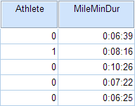
In the sample data, we will use two variables: Athlete and MileMinDur . The variable Athlete has values of either “0” (non-athlete) or "1" (athlete). It will function as the independent variable in this T test. The variable MileMinDur is a numeric duration variable (h:mm:ss), and it will function as the dependent variable. In SPSS, the first few rows of data look like this:
Before the Test
Before running the Independent Samples t Test, it is a good idea to look at descriptive statistics and graphs to get an idea of what to expect. Running Compare Means ( Analyze > Compare Means > Means ) to get descriptive statistics by group tells us that the standard deviation in mile time for non-athletes is about 2 minutes; for athletes, it is about 49 seconds. This corresponds to a variance of 14803 seconds for non-athletes, and a variance of 2447 seconds for athletes 1 . Running the Explore procedure ( Analyze > Descriptives > Explore ) to obtain a comparative boxplot yields the following graph:

If the variances were indeed equal, we would expect the total length of the boxplots to be about the same for both groups. However, from this boxplot, it is clear that the spread of observations for non-athletes is much greater than the spread of observations for athletes. Already, we can estimate that the variances for these two groups are quite different. It should not come as a surprise if we run the Independent Samples t Test and see that Levene's Test is significant.
Additionally, we should also decide on a significance level (typically denoted using the Greek letter alpha, α ) before we perform our hypothesis tests. The significance level is the threshold we use to decide whether a test result is significant. For this example, let's use α = 0.05.
1 When computing the variance of a duration variable (formatted as hh:mm:ss or mm:ss or mm:ss.s), SPSS converts the standard deviation value to seconds before squaring.
Running the Test
To run the Independent Samples t Test:
- Click Analyze > Compare Means > Independent-Samples T Test .
- Move the variable Athlete to the Grouping Variable field, and move the variable MileMinDur to the Test Variable(s) area. Now Athlete is defined as the independent variable and MileMinDur is defined as the dependent variable.
- Click Define Groups , which opens a new window. Use specified values is selected by default. Since our grouping variable is numerically coded (0 = "Non-athlete", 1 = "Athlete"), type “0” in the first text box, and “1” in the second text box. This indicates that we will compare groups 0 and 1, which correspond to non-athletes and athletes, respectively. Click Continue when finished.
- Click OK to run the Independent Samples t Test. Output for the analysis will display in the Output Viewer window.
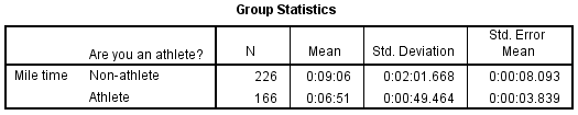
Two sections (boxes) appear in the output: Group Statistics and Independent Samples Test . The first section, Group Statistics , provides basic information about the group comparisons, including the sample size ( n ), mean, standard deviation, and standard error for mile times by group. In this example, there are 166 athletes and 226 non-athletes. The mean mile time for athletes is 6 minutes 51 seconds, and the mean mile time for non-athletes is 9 minutes 6 seconds.
The second section, Independent Samples Test , displays the results most relevant to the Independent Samples t Test. There are two parts that provide different pieces of information: (A) Levene’s Test for Equality of Variances and (B) t-test for Equality of Means.
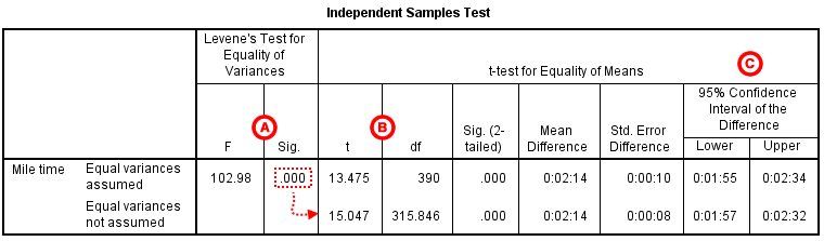
A Levene's Test for Equality of of Variances : This section has the test results for Levene's Test. From left to right:
- F is the test statistic of Levene's test
- Sig. is the p-value corresponding to this test statistic.
The p -value of Levene's test is printed as ".000" (but should be read as p < 0.001 -- i.e., p very small), so we we reject the null of Levene's test and conclude that the variance in mile time of athletes is significantly different than that of non-athletes. This tells us that we should look at the "Equal variances not assumed" row for the t test (and corresponding confidence interval) results . (If this test result had not been significant -- that is, if we had observed p > α -- then we would have used the "Equal variances assumed" output.)
B t-test for Equality of Means provides the results for the actual Independent Samples t Test. From left to right:
- t is the computed test statistic, using the formula for the equal-variances-assumed test statistic (first row of table) or the formula for the equal-variances-not-assumed test statistic (second row of table)
- df is the degrees of freedom, using the equal-variances-assumed degrees of freedom formula (first row of table) or the equal-variances-not-assumed degrees of freedom formula (second row of table)
- Sig (2-tailed) is the p-value corresponding to the given test statistic and degrees of freedom
- Mean Difference is the difference between the sample means, i.e. x 1 − x 2 ; it also corresponds to the numerator of the test statistic for that test
- Std. Error Difference is the standard error of the mean difference estimate; it also corresponds to the denominator of the test statistic for that test
Note that the mean difference is calculated by subtracting the mean of the second group from the mean of the first group. In this example, the mean mile time for athletes was subtracted from the mean mile time for non-athletes (9:06 minus 6:51 = 02:14). The sign of the mean difference corresponds to the sign of the t value. The positive t value in this example indicates that the mean mile time for the first group, non-athletes, is significantly greater than the mean for the second group, athletes.
The associated p value is printed as ".000"; double-clicking on the p-value will reveal the un-rounded number. SPSS rounds p-values to three decimal places, so any p-value too small to round up to .001 will print as .000. (In this particular example, the p-values are on the order of 10 -40 .)
C Confidence Interval of the Difference : This part of the t -test output complements the significance test results. Typically, if the CI for the mean difference contains 0 within the interval -- i.e., if the lower boundary of the CI is a negative number and the upper boundary of the CI is a positive number -- the results are not significant at the chosen significance level. In this example, the 95% CI is [01:57, 02:32], which does not contain zero; this agrees with the small p -value of the significance test.
Decision and Conclusions
Since p < .001 is less than our chosen significance level α = 0.05, we can reject the null hypothesis, and conclude that the that the mean mile time for athletes and non-athletes is significantly different.
Based on the results, we can state the following:
- There was a significant difference in mean mile time between non-athletes and athletes ( t 315.846 = 15.047, p < .001).
- The average mile time for athletes was 2 minutes and 14 seconds lower than the average mile time for non-athletes.
- << Previous: Paired Samples t Test
- Next: One-Way ANOVA >>
- Last Updated: Jul 10, 2024 11:08 AM
- URL: https://libguides.library.kent.edu/SPSS
Street Address
Mailing address, quick links.
- How Are We Doing?
- Student Jobs
Information
- Accessibility
- Emergency Information
- For Our Alumni
- For the Media
- Jobs & Employment
- Life at KSU
- Privacy Statement
- Technology Support
- Website Feedback
Conduct and Interpret an Independent Sample T-Test
What is the Independent Sample T-Test ?
The independent samples t-test is a test that compares two groups on the mean value of a continuous (i.e., interval or ratio), normally distributed variable. The model assumes that a difference in the mean score of the dependent variable is found because of the influence of the independent variable that distinguishes the two groups.
The t-test family is based on the t-distribution, because the distribution of differences in means for a normally distributed variable approximates the t-distribution. The t-test is sometimes also called Student’s t-test. Student is the pseudonym used by W.S. Gosset in 1908 in his published paper on the t-distribution based on his empirical findings on the height and the length of the left middle finger of criminals in a local prison.
The independent samples t-test compares two independent groups of observations or measurements on a single characteristic. The independent samples t-test is the between-subjects analog to the dependent samples t-test, which is used when the study involves a repeated measurement (e.g., pretest vs. posttest) or matched observations (e.g., older vs. younger siblings).

Discover How We Assist to Edit Your Dissertation Chapters
Aligning theoretical framework, gathering articles, synthesizing gaps, articulating a clear methodology and data plan, and writing about the theoretical and practical implications of your research are part of our comprehensive dissertation editing services.
- Bring dissertation editing expertise to chapters 1-5 in timely manner.
- Track all changes, then work with you to bring about scholarly writing.
- Ongoing support to address committee feedback, reducing revisions.
Examples of typical questions that the independent samples t-test answers are as follows:
- Medicine – Has the quality of life improved for patients who took drug A as opposed to patients who took drug B?
- Sociology – Are men more satisfied with their jobs than women?
- Biology – Are foxes in one specific habitat larger than in another?
- Economics – Is the economic growth of developing nations larger than the economic growth of the first world?
- Marketing : Does customer segment A spend more on groceries than customer segment B?
The Independent Samples T-Test in SPSS
Our research question for this independent samples t-test example is as follows:
Does the standardized test score for math, reading, and writing differ between students who failed and students who passed the final exam?
In SPSS, the independent samples t-test is found under Analyze > Compare Means > Independent Samples T Test …

In the dialog box of the independent samples t-test, we select the variables with our standardized test scores as the three test variables; the grouping variable is the outcome of the final exam (pass = 1 vs. fail = 0). The groups need to be defined by clicking on the button Define Groups… and entering the values of the independent variable that distinguish the groups.

The dialog box Options… allows us to define how missing cases shall be managed (either exclude them listwise or analysis by analysis). We can also define the width of the confidence interval that is used to test the difference of the mean scores in this independent samples t-test.

Statistics Solutions can assist with your quantitative analysis by assisting you to develop your methodology and results chapters. The services that we offer include:
Data Analysis Plan
Edit your research questions and null/alternative hypotheses
Write your data analysis plan; specify specific statistics to address the research questions, the assumptions of the statistics, and justify why they are the appropriate statistics; provide references
Justify your sample size/power analysis, provide references
Explain your data analysis plan to you so you are comfortable and confident
Two hours of additional support with your statistician
Quantitative Results Section (Descriptive Statistics, Bivariate and Multivariate Analyses, Structural Equation Modeling , Path analysis, HLM, Cluster Analysis )
Clean and code dataset
Conduct descriptive statistics (i.e., mean, standard deviation, frequency and percent, as appropriate)
Conduct analyses to examine each of your research questions
Write-up results
Provide APA 6 th edition tables and figures
Explain chapter 4 findings
Ongoing support for entire results chapter statistics
Please call 727-442-4290 to request a quote based on the specifics of your research, schedule using the calendar on this page, or email [email protected]
Statistics Resources
- Excel - Tutorials
- Basic Probability Rules
- Single Event Probability
- Complement Rule
- Intersections & Unions
- Compound Events
- Levels of Measurement
- Independent and Dependent Variables
- Entering Data
- Central Tendency
- Data and Tests
- Displaying Data
- Discussing Statistics In-text
- SEM and Confidence Intervals
- Two-Way Frequency Tables
- Empirical Rule
- Finding Probability
- Accessing SPSS
- Chart and Graphs
- Frequency Table and Distribution
- Descriptive Statistics
- Converting Raw Scores to Z-Scores
- Converting Z-scores to t-scores
- Split File/Split Output
- Partial Eta Squared
- Downloading and Installing G*Power: Windows/PC
- Correlation
- Testing Parametric Assumptions
- One-Way ANOVA
- Two-Way ANOVA
- Repeated Measures ANOVA
- Goodness-of-Fit
- Test of Association
- Pearson's r
- Point Biserial
- Mediation and Moderation
- Simple Linear Regression
- Multiple Linear Regression
- Binomial Logistic Regression
- Multinomial Logistic Regression
Independent Samples T-test
- Dependent Samples T-test
- Testing Assumptions
- T-tests using SPSS
- T-Test Practice
- Predictive Analytics This link opens in a new window
- Quantitative Research Questions
- Null & Alternative Hypotheses
- One-Tail vs. Two-Tail
- Alpha & Beta
- Associated Probability
- Decision Rule
- Statement of Conclusion
- Statistics Group Sessions
The independent samples t-test is used to compare two sample means from unrelated groups. This means that there are different people providing scores for each group. The purpose of this test is to determine if the samples are different from each other.
Basic Hypotheses
Null: The sample mean from Group 1 is not different from the sample mean from Group 2. Alternative: The sample mean from Group 1 is significantly different from the sample mean from Group 2.
Real-World Examples
- Is Lowfya more effective at reducing depression symptoms than DepLo?
- Do students that take the SAT Prep course score higher on the SAT than those that don't?
- Is there a difference in income based on gender?
Reporting Results in APA Style
When reporting the results of the independent-samples t-test, APA Style has very specific requirements on what information should be included. Below is the key information required for reporting the results of the. You want to replace the red text with the appropriate values from your output.
t (degrees of freedom) = the t statistic, p = p value.
Example : An independent-samples t-test was run to determine if the Mind Over Matter coping strategy was more effective at reducing anxiety than deep breathing exercises. The results showed that the participants using the Mind Over Matter strategy ( M = 21, SD = 2.2) reported lower levels of anxiety than participants using deep breathing exercises ( M = 28, SD = 2.7). This difference was significant ( t (19) = 4.37, p < .01).
- When reporting the p-value, there are two ways to approach it. One is when the results are not significant. In that case, you want to report the p-value exactly: p = .24. The other is when the results are significant. In this case, you can report the p-value as being less than the level of significance: p < .05.
- The t statistic should be reported to two decimal places without a 0 before the decimal point: .36
- Degrees of freedom for this test are ( n1 - 1) + ( n2 - 1) or ( n1 + n2 ) - 2, where " n1 " represents the number of people in one group and " n2 " represents the number of people in the other group. The n for each group can be found in the SPSS output.
Additional Resources
Laerd Statistics - Independent t-test guide Khan Academy - Testing the difference between two means
Was this resource helpful?
- << Previous: T-Test
- Next: Dependent Samples T-test >>
- Last Updated: Jul 16, 2024 11:19 AM
- URL: https://resources.nu.edu/statsresources

Thank you for visiting nature.com. You are using a browser version with limited support for CSS. To obtain the best experience, we recommend you use a more up to date browser (or turn off compatibility mode in Internet Explorer). In the meantime, to ensure continued support, we are displaying the site without styles and JavaScript.
- View all journals
- Explore content
- About the journal
- Publish with us
- Sign up for alerts
- Open access
- Published: 12 September 2024
IL-4 drives exhaustion of CD8 + CART cells
- Carli M. Stewart ORCID: orcid.org/0000-0002-2288-2230 1 , 2 , 3 ,
- Elizabeth L. Siegler 1 , 4 ,
- R. Leo Sakemura ORCID: orcid.org/0000-0002-0293-5577 1 , 4 ,
- Michelle J. Cox ORCID: orcid.org/0000-0002-2984-0834 1 ,
- Truc Huynh ORCID: orcid.org/0009-0003-7521-4185 1 , 4 ,
- Brooke Kimball ORCID: orcid.org/0009-0009-3308-2704 1 , 4 ,
- Long Mai 1 , 4 ,
- Ismail Can ORCID: orcid.org/0000-0003-0569-5326 1 , 4 ,
- Claudia Manriquez Roman 1 ,
- Kun Yun ORCID: orcid.org/0009-0000-2782-8527 1 , 2 , 5 ,
- Olivia Sirpilla ORCID: orcid.org/0000-0002-0634-407X 1 , 2 , 3 ,
- James H. Girsch 1 , 2 , 5 ,
- Ekene Ogbodo 1 , 4 ,
- Wazim Mohammed Ismail ORCID: orcid.org/0000-0002-1782-7296 6 ,
- Alexandre Gaspar-Maia ORCID: orcid.org/0000-0001-8528-5575 6 ,
- Justin Budka 7 ,
- Jenny Kim 7 ,
- Nathalie Scholler ORCID: orcid.org/0000-0003-3743-7102 7 ,
- Mike Mattie 7 ,
- Simone Filosto 7 &
- Saad S. Kenderian ORCID: orcid.org/0000-0003-2767-3830 1 , 4 , 8
Nature Communications volume 15 , Article number: 7921 ( 2024 ) Cite this article
Metrics details
- Epigenetics in immune cells
- Interleukins
- Translational immunology
- Translational research
Durable response to chimeric antigen receptor T (CART) cell therapy remains limited in part due to CART cell exhaustion. Here, we investigate the regulation of CART cell exhaustion with three independent approaches including: a genome-wide CRISPR knockout screen using an in vitro model for exhaustion, RNA and ATAC sequencing on baseline and exhausted CART cells, and RNA and ATAC sequencing on pre-infusion CART cell products from responders and non-responders in the ZUMA-1 clinical trial. Each of these approaches identify interleukin (IL)-4 as a regulator of CART cell dysfunction. Further, IL-4-treated CD8 + CART cells develop signs of exhaustion independently of the presence of CD4 + CART cells. Conversely, IL-4 pathway editing or the combination of CART cells with an IL-4 monoclonal antibody improves antitumor efficacy and reduces signs of CART cell exhaustion in mantle cell lymphoma xenograft mouse models. Therefore, we identify both a role for IL-4 in inducing CART exhaustion and translatable approaches to improve CART cell therapy.
Introduction
Chimeric antigen receptor T (CART) cell therapy has evolved as a potentially curative therapy in a subset of patients with hematological malignancies 1 . While CART cell therapy results in impressive overall response rates over 70%, durable response rates remain limited to 30–40%, and most patients relapse within the first year of therapy 2 , 3 , 4 . Several mechanisms of CART cell failure have been identified, including the limited in vivo expansion and persistence of CART cells 5 , 6 .
It has become increasingly evident that T cell exhaustion contributes to CART cell failure in the clinic 7 , 8 . T cell exhaustion is an epigenetically regulated state of dysfunction that results from chronic stimulation through either the T cell receptor (TCR) in CD8 + T cells or through the CAR in CART cells 9 , 10 , 11 , 12 . Exhaustion is characterized by phenotypic, functional, transcriptional, and epigenetic changes. Phenotypic alterations include the upregulation of multiple inhibitory receptors on a cell such as programmed cell death protein 1 (PD-1), T cell immunoglobulin and mucin domain-containing protein 3 (TIM-3), cytotoxic T-lymphocyte associated protein 4 (CTLA-4), and lymphocyte-activation gene 3 (LAG-3) 9 . Functional alterations include a decreased ability to proliferate and to produce effector cytokines such as interleukin (IL)-2 and tumor necrosis factor (TNF)-α, followed by losing the ability to produce interferon (IFN)-γ at later stages 9 . In addition, exhausted T cells experience metabolic changes such as impaired glycolysis 13 . Transcriptional and epigenetic changes include alterations in the activity of several transcription factors including: TCF-7, TOX, T-BET, EOMES, PRDM1, NR4A3, BATF, and EGR2, as well as AP-1 and RUNX family members 14 , 15 , 16 , 17 , 18 , 19 , 20 , 21 , 22 , 23 , 24 , 25 , 26 . In an effort to control the epigenetic response to chronic stimulation, several studies have used genetic engineering tools to overexpress or knockout individual molecules. Some examples include the overexpression of the AP-1 family member c-Jun and the deletion of molecules such as the methyltransferase DNMT3A, the inflammatory regulators REGNASE-1 and ROQUIN-1, and the transcription factors PRDM1 and NR4A3 11 , 25 , 27 , 28 . While these approaches have both enhanced the field’s understanding of CART cell exhaustion as well as established a framework to prevent its development, a complete understanding of molecular pathways and potential targets for therapeutic intervention has not been achieved thus far.
It is likely that the occurrence of CART cell exhaustion varies by CAR construct and disease type. For example, independent studies have demonstrated that CD28-costimulated CART cells are more susceptible to a state of exhaustion as compared to 41BB-costimulated CART cells 5 , 29 , 30 . In addition, CAR constructs that experience a higher occurrence of tonic signaling have also been positively associated with the development of CART cell exhaustion 29 . Further, current literature supports a higher risk of exhaustion in CART cells used for the treatment of solid tumors due to the added challenges of an immunosuppressive tumor microenvironment 31 .
We focused our studies on the epigenetic regulation of exhaustion in CART cells targeting the CD19 antigen (CART19) and containing a CD28 costimulatory domain (CART19-28ζ) as a model. To do so, we employed the following three independent strategies: (1) a genome-wide clustered regularly interspaced short palindromic repeat (CRISPR) knockout screen in healthy donor CART19-28ζ cells using an in vitro model for exhaustion, (2) RNA and assay for transposase-accessible chromatin (ATAC) sequencing on baseline and chronically stimulated CART19-28ζ cells from healthy donors using an in vitro model for exhaustion, and (3) RNA and ATAC sequencing on pre-infusion axicabtagene ciloleucel (axi-cel) products from patient responders and non-responders in the pivotal ZUMA-1 clinical trial that led to the initial FDA approval of axi-cel 32 . Collectively, our independent approaches identified IL-4 as a key regulator of CART cell exhaustion. Subsequently, we performed validation studies to confirm the role of IL-4 on CART cell function using in vitro and in vivo models, ultimately proposing IL-4 neutralization as a strategy to improve CART cell anti-tumor activity.
Establishing an in vitro model for CART19 cell exhaustion
To better understand the development of CART cell exhaustion, we first designed an in vitro model to induce exhaustion in CART19 cells generated from healthy donor T cells (Fig. 1a and Supplementary Fig. S1 ). This model was designed both to be scalable and to focus specifically on the development of exhaustion through chronic stimulation of the T cells. In CD8 + T cells, exhaustion has been modeled in vitro by the chronic stimulation of the T cells through the T cell receptor (TCR) 9 , 33 . To model this phenomenon in CART19-28ζ cells, we chronically stimulated CART cells through the CAR with the addition of fresh CD19 + target cells to the culture every other day. When CART19-28ζ cells were chronically stimulated with the CD19 + mantle cell lymphoma cell line, JeKo-1, they became progressively dysfunctional as evident by reduced CART cell antigen specific expansion in vitro (Fig. 1b ). Additionally, chronically stimulated CART cells exhibited phenotypical and functional signs of exhaustion such as the increased co-expression of multiple inhibitory receptors and the decreased production of effector cytokines such as IL-2 and TNF-α (Supplementary Fig. S2a–d ). Furthermore, these cells exhibited reduced polyfunctionality as determined by the number of T cells secreting three or more cytokines (Supplementary Fig. S2e ). Importantly, changes in antigen specific expansion, the co-expression of inhibitory receptors, and the production of effector cytokines appear to be a result of chronic stimulation and not due to a change in the percentage of CAR + T cells (Supplementary Fig. S2f ) or due to long-term co-culture (Supplementary Fig. S3 ).

a Schematic depicting an in vitro model for exhaustion in CART cells (Fig. 1a was created with BioRender.com released under a Creative Commons Attribution-NonCommercial-NoDerivs 4.0 International license). b Absolute CD3 + cell count, as determined with flow cytometry, after Day 8 (baseline), Day 15 (1 week of chronic stimulation), and Day 22 (2 weeks of chronic stimulation) CART19-28ζ cells were co-cultured with JeKo-1 target cells at a 1:1 ratio for 5 days (One-way ANOVA with average of two technical replicates for three biological replicates, mean ± standard deviation (SD)). c In vivo antitumor activity of Day 22 and Day 8 CART19-28ζ cells in a JeKo-1 xenograft model. NOD-SCID-IL2rγ−/− (NSG) mice were engrafted with the CD19 + luciferase + JeKo-1 cells (1 x 10 6 cells I.V.). Mice underwent bioluminescent imaging weekly to confirm engraftment and to monitor tumor burden. Total flux is depicted over time following treatment with CART19-28ζ (0.9 x 10 6 cells I.V.) on Day 0 (Two-way ANOVA, n = 5 mice per group, mean ± SD). d Overall survival curve based on JeKo-1 xenograft mouse model comparing treatment with Day 8 or Day 22 CART19-28ζ cells (Log-rank (Mantel–Cox) test, n = 5 mice per group) e Bioluminescent imaging of the tumor growth in the JeKo-1 xenograft mouse model. f In vivo CART cell expansion as determined by absolute count of hCD45 + CD3 + cells per μL of blood by flow cytometry on Day 15 of the JeKo-1 xenograft model. (two-sided t test, n = 5 mice per group, mean ± SD) g Circle graphs showing the average portion of CART cells expressing multiple inhibitory receptors (0—black, 1—pink, 2—green, 3—dark purple) based on flow cytometry detection of PD-1, CTLA-4, and TIM-3 on human CD3 + cells in the peripheral blood of mice on Day 15 of the JeKo-1 xenograft model. (Average portion from n = 5 mice per group) h – j Human cytokine levels for IL-2, IFN-γ, and IL-10 as determined by Multiplex bead assay of mouse serum collected from peripheral blood on Day 15 of the JeKo-1 xenograft model. (two-sided t test, n = 5 mice per group, mean ± SD). Source data for ( b – d ) and ( f – j ) are provided in the Source Data file.
To further examine the function and phenotype of chronically stimulated CART cells, we utilized a mantle cell lymphoma xenograft mouse model that stress tests CART19 cells (Supplementary Fig. S4a ). In this model, mice are allowed to develop high disease burden so that standard CART19 doses fail to induce a complete remission of the tumor. Mice were then randomized to receive treatment with either baseline (Day 8) or chronically stimulated (Day 22) CART19-28ζ cells. Treatment with chronically stimulated CART19-28ζ cells resulted in a significant reduction in anti-tumor activity (Fig. 1c and Supplementary Fig. S4b ) and overall survival (Fig. 1d, e and Supplementary Fig. S4c ), compared to treatment with baseline CART19-28ζ. In addition, there was a trend for decreased CART expansion (Fig. 1f and Supplementary Fig. S4d ) and a significant upregulation of multiple inhibitory receptors (Fig. 1g and Supplementary Fig. S4e, f ) on CART cells in the peripheral blood of mice treated with chronically stimulated CART19-28ζ cells. Further, peripheral blood cytokine analysis two weeks following CART cell injection showed significantly decreased levels of several effector cytokines (Supplementary Fig. S4g ), including IL-2 (Fig. 1h ) and IFN-γ (Fig. 1i ), in mice treated with chronically stimulated CART cells. These mice also showed significantly elevated levels of the inhibitory cytokine IL-10 (Fig. 1j ). These findings corroborate our in vitro data and align with an exhausted phenotype.
Having demonstrated that our in vitro model for CART cell exhaustion leads to phenotypic and functional changes associated with T cell exhaustion, we next tested whether this model is applicable to other tumor models and CAR constructs. Consistent with our initial data, chronic stimulation of CART19-28ζ cells with the CD19 + acute lymphoblastic leukemia cell line, NALM-6 (Supplementary Fig. S5 ), or chronic stimulation of 4-1BB-costimulated CART19 (CART19-BBζ) cells with JeKo-1 cells (Supplementary Fig. S6 ) resulted in functional and phenotypical signs of T cell exhaustion. As such, our in vitro model is a representative model for inducing CART cell exhaustion in different tumor models and different CAR constructs.
CRISPR screen identifies a role for the IL-4 pathway in CART failure
To investigate genes and pathways that can be altered to protect CART cells from exhaustion, we conducted a genome-wide CRISPR knockout screen using healthy donor CART19-28ζ cells. To do this, we scaled our in vitro model for CART cell exhaustion by transducing 1 × 10 8 CART cells with the GeCKO v2 library A on Day 2 at a multiplicity of infection (MOI) of 0.3 (Fig. 2a ) 34 . Then, we selected for transduced cells through treatment with puromycin from Day 3 to Day 8.

a Schematic depicting the in vitro genome-wide CRISPR knockout screen conducted in healthy donor CART19-28ζ cells (Fig. 2a was created with BioRender.com released under a Creative Commons Attribution-NonCommercial-NoDerivs 4.0 International license). b The Gini index on Day 8 and Day 22 of the CRISPR screen (Gini index was calculated with MAGeCK-VISPR and compared with a two-sided t test, three biological replicates). c Principal component analysis plot of gRNA representation in the CRISPR screen at Day 8 and Day 22 (MAGeCK-VISPR maximum likelihood estimation (MLE) analysis with three biological replicates). d Volcano plot showing genes that were positively (red) or negatively (green) selected by Day 22 of the CRISPR screen as compared to Day 8 (Results from MAGeCK-VISPR MLE analysis with three biological replicates). e Top pathways identified by gene ontology enrichment analysis of the positively selected genes (FDR < 0.25 as determined with MAGeCK-VISPR analysis with three biological replicates). f Average fold-change of IL-4 gRNA representation from Day 8 to Day 22 of the CRISPR screen from three biological replicates (fold change calculated with normalized counts of IL-4 targeting gRNAs as determined with MAGeCK-MLE with three biological replicates). Source data for ( b ) and ( f ) are provided in the Source Data file.
By Day 22 of the chronic stimulation assay, we observed positive selection of guide RNAs (gRNAs) as seen by an increase in the Gini index from Day 8 to Day 22 (Fig. 2b ) and principal component analysis (PCA) (Fig. 2c ). Additionally, there were little changes in the presence of non-targeting gRNAs from Day 8 to Day 22 of the CRISPR screen (Supplementary Fig. S7a ). However, to adequately assess changes in gRNA representation throughout the screen, we normalized all gRNA counts to counts from the list of 1000 non-targeting gRNAs. To further verify the quality of the CRISPR screen, we examined the top negatively and positively selected genes. Top results from gene set enrichment analysis of the negatively selected genes include pathways associated with ribosomal genes and translational processes (Supplementary Fig. S7b ). This is expected as knockout of these pathways leads to a strong negative selection phenotype 35 . Among the top positively selected genes, there are several genes that have previously been associated with CART cell dysfunction ( CSF2 , SOCS1 , and PTPN2 ) (Fig. 2d ). Knockout of these genes with CRISPR Cas9 in previously published studies has resulted in increased proliferative ability and decreased signs of CART cell dysfunction 36 , 37 , 38 , 39 . Together, these data indicate that the genome-wide CRISPR knockout screen effectively identified positively, and negatively selected genes associated with CART cell dysfunction.
To investigate key pathways associated with CART cell exhaustion, we performed gene ontology enrichment analysis on the list of positively selected genes. This analysis revealed a role for several cytokine signaling pathways in CART cell exhaustion including the IFN-γ, IL-2, and IL-4 pathways (Fig. 2e ). In an independent causal network analysis of the positively selected genes with QIAGEN ingenuity pathway analysis (IPA), the IL-4 receptor (IL4R) was identified as a top regulator (Supplementary Fig. S8 ). Upon closer investigation of the gRNAs targeting IL-4 in the screen, two out of the three gRNAs targeting IL-4 had enhanced representation in the chronically stimulated (Day 22) samples as compared to baseline (Day 8) samples (Fig. 2f ). This suggests that the IL-4 pathway is involved in CART cell exhaustion.
IL-4 is involved in regulation of exhaustion
To further interrogate the top pathways identified with the genome-wide CRISPR knockout screen, and to enhance the field’s understanding of the epigenetic regulation of CART cell exhaustion, we interrogated the transcriptome and chromatin accessibility pattern of baseline and chronically stimulated CART19-28ζ cells from our in vitro model for exhaustion. RNA sequencing of baseline (Day 8) and chronically stimulated (Day 15) CART19-28ζ cells revealed the development of a distinct transcriptomic profile (Fig. 3a ). Several genes that have previously been correlated with an exhausted phenotype, such as EOMES , IL10RA , and HAVCR2 (TIM-3), were confirmed to be upregulated in chronically stimulated CART19-28ζ cells (Fig. 3b ). Additionally, the transcription of AP-1 family members that have previously been negatively correlated with the development of exhaustion, such as FOS and FOSL2 , were downregulated (Fig. 3b ) 27 . These findings further validate the development of CART exhaustion in our model.

a , b Heat map and volcano plot showing differentially expressed genes when comparing chronically stimulated (Day 15) to baseline (Day 8) CART19-28ζ cells (DESEQ2 with three biological replicates, padj < 0.05). In the volcano plot, significantly differentially expressed genes (padj < 0.05) are colored red. c Top differentially regulated pathways as determined by QIAGEN IPA of differentially expressed genes (DESEQ2 with three biological replicates, padj < 0.05). d , e Motifs enriched in chronically stimulated as compared with baseline CART19-28ζ cells (MEME/TOMTOM analysis with three biological replicates). f , g Top canonical pathways and upstream regulators as identified by QIAGEN IPA of genes that were both differentially expressed (DESEQ2 with three biological replicates, padj < 0.05) and differentially accessible (DiffBind with DESEQ2 using three biological replicates, padj < 0.05). h Ratio of CD4 + to CD8 + CART19-28ζ cells in baseline (Day 8) and chronically stimulated (Day 15) cell populations from the in vitro model for exhaustion (Paired two-sided t test, average of two technical replicates for three biological replicates, mean ± SD). i The percent of CD4 + CART19-28ζ cells that are Th2 polarized as determined by CCR6 - CCR4 + CXCR3 - via flow cytometry in baseline (Day 8) and chronically (Day 15) stimulated CART19-28ζ cell populations (Paired two-sided t test, average of two technical replicates for three biological replicates, mean ± SD). j The percent of either CD3 + , CD4 + , or CD8 + CART19-28ζ cells producing IL-4 as determined by intracellular staining for IL-4 by flow cytometry following four hours of antigen-specific CAR stimulation through co-culturing Day 8 or Day 15 CART19-28ζ cells with JeKo-1 cells at a 1:5 effector-to-target (E:T) cell ratio (Two-way ANOVA, average of two technical replicates for three biological replicates, mean ± SD). Source data for ( h – j ) are provided in the Source Data file.
To determine the activity of signaling pathways during the development of exhaustion, we performed pathway analysis using both the list of differentially expressed genes and their respective fold changes. This analysis revealed a strong downregulation in pathways associated with metabolism such as glycolysis and gluconeogenesis and highlighted the importance of cytokine signaling in the development of exhaustion (Fig. 3c ).
Next, we performed ATAC sequencing on baseline (Day 8) and chronically stimulated (Day 15) CART19-28ζ cells to investigate the epigenetic changes responsible for the development of exhaustion. Consistent with the transcriptomic changes and existing literature, there was enhanced chromatin accessibility at exhaustion-related gene loci (e.g., PDCD1 and ENTPD1 ) in our chronically stimulated samples (Supplementary Fig. S9a, b ) as well as enhanced motif accessibility for AP-1 and RUNX family members (Fig. 3d, e ) 27 , 33 .
After verifying that known transcriptomic and epigenetic changes associated with exhaustion are seen following chronic stimulation of CART cells in our in vitro model for exhaustion, we next asked how the development of exhaustion was being regulated. To uncover epigenetic regulators of CART cell exhaustion, we overlapped the genes that were both differentially expressed and differentially accessible. Then, using QIAGEN IPA, we evaluated top affected pathways and upstream regulators by using both the list of overlapped genes and their respective fold changes, as determined with RNA sequencing. The top enriched pathway was the T cell exhaustion pathway (Fig. 3f ). Other pathways with indeterminant enrichment statuses include pathways involved with Th1, Th2 or T helper cell activation or differentiation (Fig. 3f ). Top predicted upstream regulators include IL-2, IL-15, TCF-7, ITK, and IL-4 (Fig. 3g ). IL-2, IL-15, TCF-7 and ITK have previously been linked to the development of T cell exhaustion 9 , 16 , 40 , 41 , 42 . However, while IL-4 has classically been associated with Th2 polarization in CD4 + T cells, its role in the development of CART cell exhaustion has not been well-studied.
IL-4 production in CD8 + CART cells increases upon chronic stimulation
Given both the identification of IL-4 as a top upstream regulator in the development of exhaustion and the inclusion of pathways related to T helper cell differentiation in the top affected pathways, we asked whether IL-4 was identified as a top upstream regulator as a result of changes in the T helper cell polarization or as a result of the development of exhaustion.
To approach this question, we utilized multiple independent approaches to differentiate T cell exhaustion from T helper cell polarization in our in vitro model for CART cell exhaustion. First, we observed a sharp decrease in the CD4 + population of CART19-28ζ cells following chronic stimulation, an established finding during the development of exhaustion (Fig. 3h ) 9 . Second, we inspected the Th1 and Th2 populations of cells within the declining CD4 + population and observed a significant decrease in the Th2 population within the CD4 + cells (Fig. 3i) and an increase in the Th1 population (Supplementary Fig. S10a ). Third, we evaluated the serum cytokine levels of the Th2 cytokines IL-5 and IL-13 in JeKo-1 xenograft mice treated with either baseline (Day 8) or chronically stimulated (Day 22) CART19-28ζ cells and observed a reduction in the levels of these cytokines in mice treated with chronically stimulated CART19-28ζ cells (Supplementary Fig. S10b, c ). Fourth, we observed an increase in IL-4 production in CART19-28ζ cells following chronic stimulation with JeKo-1 cells (Fig. 3j ). Notably, there was a significant increase in IL-4 production in CD8 + CART19-28ζ cells, but not in CD4 + CART19-28ζ cells (Fig. 3j ).
Overall, IL-4 was identified as a top upstream regulator of exhaustion based on epigenetic changes observed from Day 8 to Day 15 of our in vitro model for exhaustion. While this model also produces a shift in the T helper cell population, the shift is towards a Th1 population. This is unexpected given the role of IL-4 in polarizing CD4 + T cells towards a Th2 phenotype. However, we believe IL-4 is mainly identified as a top upstream regulator as a result of its impact on the CD8 + population of CART cells. This is supported by both an increase in the production of IL-4 by CD8 + CART cells and a significant reduction in CD4 + CART cells following chronic stimulation.
IL-4 is enriched in CART cell products from non-responders
Next, we aimed to determine the significance of our findings in patients treated with CART19-28ζ cells. We interrogated the transcriptome and chromatin accessibility pattern of pre-infusion axi-cel products from responders and non-responders in the pivotal ZUMA-1 clinical trial that led to the initial FDA approval of axi-cel 32 . In this analysis, responders were defined as patients who achieved complete remission as best response while non-responders were defined as patients who experienced stable or progressive disease. There was no observed difference in the percent of T cells expressing CAR between responders and non-responders (Supplementary Fig. S11a ).
Interrogation of the transcriptome with RNA sequencing of pre-infusion axi-cel products from 6 responders and 6 non-responders showed clustering of non-responder samples (Fig. 4a ). The top upregulated genes in non-responders include IL-4 and CCR3, a chemokine receptor that is known to be induced by IL-4 and IL-2 (Fig. 4b ) 43 . Additionally, analysis of the differentially expressed genes with QIAGEN IPA identified IL-4 as one of the upstream regulators, along with other genes such as TNF and STAT3 (Fig. 4c ). Interestingly, when we evaluate changes in chromatin accessibility between baseline axi-cel products from responders and non-responders, we see many similarities to the findings observed following chronic stimulation of healthy donor CART19-28ζ cells in our in vitro model for exhaustion. Motif analysis revealed an enrichment of motif binding sites for EOMES and PRDM1 (Fig. 4d, e ). Both of these transcription factors have previously been associated with the development of exhaustion 22 , 23 . Additionally, non-responders showed similar enhancement of chromatin accessibility to exhausted cell populations at exhaustion-related gene loci such as PDCD1 , HAVCR2 (TIM-3), EOMES , and IL-10 (Supplementary Fig. S12a–d ). These findings indicate that epigenetic changes in baseline CART cell products contribute to CART cell exhaustion and failure in the clinic.

a , b Heat map and volcano plot showing differentially expressed genes when comparing pre-infusion axi-cel products from non-responders to pre-infusion axi-cel products from responders (DESEQ2, six biological replicates per condition, p < 0.05). In the volcano plot, significantly differentially expressed genes ( p < 0.05) are colored red. c Top upstream regulators as determined by QIAGEN IPA of differentially expressed genes between non-responder and responder samples (DESEQ2, six biological replicates per condition, p < 0.05). d , e Enriched motifs in pre-infusion products from non-responders as compared to pre-infusion products from responders (MEME/TOMTOM analysis with six biological replicates per condition). f ATAC signal track of IL-4 gene locus from averaged signal for each experimental condition (axi-cel products from non-responders ( n = 6), axi-cel products from responders ( n = 6), Day 15 CART19-28ζ cells ( n = 3), and Day 8 CART19-28ζ cells ( n = 3)) as visualized with the UCSC genome browser.
Looking more specifically at the IL-4 locus, we see enhanced chromatin accessibility in non-responder samples as compared to responders (Fig. 4f ). The chromatin accessibility pattern mirrors the change in accessibility observed when healthy donor CART19-28ζ cells are chronically stimulated. In particular, there is enhanced accessibility in both non-responder and chronically stimulated samples at a hypersensitivity site in intron 2 (Fig. 4f ). This site correlates with an enhancer locus for IL-4, HS2, that specifically regulates IL-4 without impacting other Th2 cytokines 44 . Collectively, these data indicate that IL-4 regulation in non-responders is consistent with changes seen following the development of CART cell exhaustion in our in vitro model for exhaustion.
IL-4 induces exhaustion independently of the presence of CD4 + CART cells
Due to our identification of IL-4 as a key regulator of CART cell exhaustion through three independent approaches, we performed in vitro studies to directly evaluate phenotypic and functional changes that occur when CART19-28ζ cells are treated with human recombinant IL-4 (hrIL-4). In addition, we also performed experiments to determine if IL-4 regulates CART cell function independently of CD4 + CART cells.
Upon stimulating either bulk (CD3 + ) or CD8 + CART19-28ζ cells once with JeKo-1 target cells in the presence of 20 ng/mL hrIL-4 (vs. diluent), CART19-28ζ cells showed signs of dysfunction such as reduced cytotoxicity (Fig. 5a ) and reduced proliferative ability as determined through CFSE staining (Supplementary Fig. S13a ). These changes appear to be independent of a direct impact of hrIL-4 on JeKo-1 cells as treatment of JeKo-1 cells with hrIL-4 alone did not affect their growth or survival (Supplementary Fig. S13b ). Additionally, these changes appear to be independent of a change in the percentage of CAR + T cells as treatment of CART cells with hrIL-4 does not change CAR expression (Supplementary Fig. S13c ).

a Percent killing as measured with bioluminescent imaging after Day 8 CD3 + or CD8 + CART19-28ζ cells were co-cultured with luciferase + JeKo-1 cells at various E:T cell ratios for 48 hours in the presence of either 20ng/mL human recombinant IL-4 (hrIL-4) or diluent (Two-way ANOVA, average of two technical replicates for three biological replicates, mean ± SD). b , f CD3 + and CD8 + CART19-28ζ cells were kept in media supplemented with 100 IU/mL hrIL-2 and chronically stimulated from Day 8 to Day 15 of the in vitro model for exhaustion in the presence of either 20ng/mL hrIL-4 or diluent control. b Absolute CD3 + cell count as measured with flow cytometry after Day 15 CART19-28ζ cells were co-cultured with JeKo-1 cells at a 1:1 E:T cell ratio for five days. (Two-way ANOVA, average of two technical replicates for three biological replicates). c , d The percent of CD3 + cells producing IL-2 and IFN-γ as determined with intracellular staining and flow cytometry after Day 15 CART19-28ζ cells were co-cultured with JeKo-1 cells at a 1:5 E:T cell ratio for four hours (Two-way ANOVA, average of two technical replicates for three biological replicates). e The percent of CART19-28ζ cells co-expressing multiple inhibitory receptors (0—black, 1—pink, 2—green, 3—dark purple, 4—light purple) on Day 15 as determined by flow cytometric detection of PD-1, CTLA-4, TIM-3, and LAG-3 on CD3 + cells (Circle plots from one representative biological replicate). f The change in the transcription of EOMES as determined with RT-qPCR of Day 15 CD3 + or Day 15 CD8 + CART19-28ζ cells (Paired two-sided t-tests average of two technical replicates for three biological replicates, mean ± SD). Source data are provided as a Source Data file.
Next, we sought to evaluate the impact of IL-4 on CART19-28ζ cells in the presence of chronic stimulation using our in vitro model for CART cell exhaustion. Upon chronic stimulation of either bulk or CD8 + CART19-28ζ cells in the presence of 20 ng/mL hrIL-4 (vs. diluent), CART19-28ζ cells showed enhanced functional and phenotypic signs of exhaustion such as (1) reduced expansion (Fig. 5b ), (2) reduced production of effector cytokines such as IL-2 and IFN-γ (Fig. 5c, d and Supplementary Fig. S13d, e ), and (3) an increase in the percent of cells coexpressing inhibitory receptors (Fig. 5e and Supplementary Fig. S13f, g ). The increase in the coexpression of inhibitory receptors appears to be dose-dependent with the greatest increase seen at the highest dose of hrIL-4 tested, 20 ng/mL (Supplementary Fig. S13h ).
With evidence that IL-4 induces CART cell exhaustion independently of CD4 + CART cells, we next investigated the transcriptional changes responsible for IL-4-induced CART cell dysfunction. Given that 1) a prior study in CD8 + T cells showed the induction of the transcription factor EOMES by IL-4 45 and that 2) EOMES is enriched in both chronically stimulated healthy donor CART cells and non-responder axi-cel products, we asked whether treatment of CART19-28ζ cells with hrIL-4 would induce the expression of EOMES. After chronically stimulating either bulk or CD8 + CART19-28ζ cells in the presence of hrIL-4, EOMES transcription is induced as compared to the diluent-treated group (Fig. 5f ).
Next, to evaluate if IL-4-induced CART cell dysfunction is dependent on additional interactions between the CART19-28ζ cells and target cells, we evaluated functional and phenotypical changes when CART19-28ζ cells are chronically stimulated with CD19-conjugated beads in the presence of either hrIL-4 or diluent. In this tumor-free assay, chronic stimulation of CART19-28ζ in the presence of hrIL-4 enhances the exhaustion profile as seen by (1) decreased production of IL-2, (2) increased coexpression of inhibitory receptors, and (3) decreased CART cell expansion (Supplementary Fig. S14a–d ). This suggests that IL-4-induced CART cell exhaustion is due to a direct effect on CART cells and is independent of CART-tumor interactions.
Given the direct effect of hrIL-4 on CART19-28ζ cells, we next assessed if hrIL-4 induces CART cell exhaustion in different CAR constructs and tumor models. To test this, we generated a variety of CART cells by using CAR constructs that are similar to the constructs used in the clinic, including 1) CART19-BBζ, 2) BCMA-targeting 4-1BB-costimulated CART cells (BCMA CART-BBζ), and 3) CS1-targeting CD28-costimulated CART cells (CS1 CART-28ζ) (Supplementary Fig. S1b ) 46 , 47 , 48 , 49 . Chronic stimulation of CART19-BBζ with JeKo-1 cells (Supplementary Fig. S15 ), BCMA CART-BBζ with OPM-2 multiple myeloma cells (Supplementary Fig. S16 ), or CS1 CART-28ζ with OPM-2 cells (Supplementary Fig. S17 ) in the presence of hrIL-4 enhanced the exhaustion phenotype. These data indicate that IL-4 supplementation can drive CART cell exhaustion independent of construct design or tumor models.
IL-4 neutralization improves the longevity and efficacy of CART cells
Given that IL-4 induces signs of CART cell exhaustion, we next examined whether disrupting the IL-4 pathway in CART cells with gene editing could reduce the prevalence of exhaustion. To start, we used CRISPR Cas9 to create IL-4 knockdown CART cells. Using two separate gRNAs, we were able to create targeted mutations to reduce CART19-28ζ production of IL-4 upon stimulation with CD19 + JeKo-1 cells (Supplementary Fig. S18a, b ). At baseline, IL-4 knockdown CART19-28ζ cells showed enhanced cytotoxicity (Supplementary Fig. S18c, d ) as compared with control gRNA CART19-28ζ cells. IL-4 knockdown CART cells also showed reduced phenotypical and functional signs of exhaustion following chronic stimulation such as (1) increased CART expansion (Supplementary Fig. S18e, f ), (2) increased production of effector cytokines such as IL-2 and IFN-γ (Supplementary Fig. S18g–i ), and (3) reduced co-expression of multiple inhibitory receptors (Supplementary Fig. S18j ).
Importantly, IL-4 knockdown did not significantly alter the CD4-to-CD8 ratio at baseline or following chronic stimulation (Supplementary Fig. S19a–c ). This indicates that IL-4’s role in driving CART cell exhaustion is not due to a change in the CD4-to-CD8 ratio. Further, given our previous finding that IL-4 supplementation can drive an exhausted phenotype in CD8 + CART cells, we looked at functional and phenotypical changes in CD8 + CART cells following chronic stimulation of IL-4 knockdown CART19-28ζ cells with JeKo-1 cells. IL-4 knockdown appears to reduce the exhausted phenotype of CD8 + CART19-28ζ cells as seen by an increase in the production of effector cytokines such as IL-2 and IFN-γ (Supplementary Fig. S20a–c ) and a reduction in the co-expression of multiple inhibitory receptors (Supplementary Fig. S20d ).
Next, to further evaluate if IL-4 reception by CART cells can drive an exhausted phenotype, we generated IL4R knockdown CART19-28ζ cells by using CRISPR Cas9 (Supplementary Fig. S21a ). Following chronic stimulation with JeKo-1 cells, IL4R knockdown CART cells showed reduced phenotypical and functional signs of exhaustion such as (1) increased proliferative ability (Supplementary Fig. S21b ), (2) decreased co-expression of multiple inhibitory receptors (Supplementary Fig. S21c ), and (3) increased production of effector cytokines (Supplementary Fig. S21d, e ). Further, the CD8 + population of IL4R knockdown CART cells also showed reduced phenotypical and functional signs of exhaustion (Supplementary Fig. S22 ). This further supports the notion that IL-4 can drive an exhausted phenotype in CD8 + CART cells.
To validate our in vitro findings that IL-4 pathway editing can improve the activity of CART19-28ζ cells, we also tested IL-4 and IL4R knockdown CART cells in vivo. We utilized a CD19 + JeKo-1 stress xenograft mouse model, similar to the one previously described (Supplementary Fig. S23a ). In this model, both IL-4 and IL4R knockdown CART cells showed improved antitumor activity as compared with control gRNA CART19-28ζ cells (Supplementary Fig. S23b ). Additionally, IL-4 and IL4R knockdown CART cells appeared to expand more in vivo (Supplementary Fig. S23c ). This indicates that editing of the IL-4 pathway in CART cells can improve the activity of CART cells both in vitro and in vivo.
While CRISPR editing of the IL-4 pathway showed promise both in vitro and in vivo, we also decided to explore the use of an IL-4 monoclonal antibody (mAb) to neutralize IL-4. This represents a translatable strategy to improve CART cell outcomes in the clinic, as there are currently available, FDA-approved IL-4 mAbs 50 , 51 , 52 .
The addition of 10 μg/mL of a commercially available IL-4 mAb (clone MP4-25D2) in co-cultures of CART19 and JeKo-1 cells showed complete neutralization of IL-4 (Supplementary Fig. S24a ) and an increase in cytotoxicity (Supplementary Fig. S24b ) as compared to treatment with an IgG control antibody. Further, when CART19-28ζ cells are chronically stimulated in the presence of 10 μg/mL IL-4 mAb, there is a significant decrease in the percent of CART19-28ζ cells that express the inhibitory receptor PD-1 (Supplementary Fig. S24c ). Chronic stimulation of CART19-28ζ cells in the presence of 10 µg/mL IL-4 mAb does not significantly alter the percentage of CAR + T cells (Supplementary Fig. S24d ).
To further investigate the combination of CART19-28ζ cells with an IL-4 mAb, we used our CD19 + JeKo-1 stress xenograft mouse model (Fig. 6a ), similar to the one depicted in Supplementary Fig. S3a . Following CART cell injection, mice were randomized based on tumor burden to weekly intraperitoneal (i.p.) injections of either 10 mg/kg IL-4 mAb or an IgG control antibody for 5 weeks. In this model, the majority of mice treated with CART19-28ζ cells and an IgG control antibody were unable to effectively clear their tumor burden (Fig. 6b, c ). In contrast, all mice treated with a combination of CART19-28ζ cells and an IL-4 mAb were able to effectively clear their tumor burden and delay tumor relapse (Fig. 6b, c ). Thus, combining CART19-28ζ cells with an IL-4 mAb resulted in enhanced antitumor activity (Fig. 6b, c ) and a trend for prolonged overall survival (Fig. 6d ).

a Schema for mantle cell lymphoma xenograft mouse model in NSG mice used to test the treatment efficacy of CART19-28ζ cells combined with 10mg/kg IL-4 monoclonal antibody (mAb) as compared with CART19-28ζ combined with 10mg/kg IgG control antibody (Fig. 6a was created with BioRender.com released under a Creative Commons Attribution-NonCommercial-NoDerivs 4.0 International license). b , c Tumor progression as monitored by bioluminescence imaging over time following injection of CART cells on Day 0 (Two-way ANOVA, n = 5 mice per group, mean ± SD). d Overall survival curve comparing CART19-28ζ cell treatment combined with either an IL-4 mAb or IgG control antibody (Log-rank (Mantel–Cox) test, n = 5 mice per group). e Absolute hCD45 + CD3 + cells per μL of blood on Day 15 of the in vivo study as determined by flow cytometric measurement of cells that are human CD45 + and human CD3 + after collecting peripheral blood via tail vein bleeding (two-sided t test, n = 5 mice per group, mean ± SD). f Circle graph showing the average portion of CART cells positive for multiple inhibitory receptors (0—black, 1—pink, 2—green, 3—dark purple) as determined with flow cytometric detection of human CD3 + cells positive for PD-1, TIM-3, and/or CTLA-4 in the peripheral blood of mice on Day 15 of the in vivo study (Average value from n = 5 mice per group). g The concentration of IL-10 in the serum of mice in the in vivo model two weeks after the injection of CART cells. Serum was collected through tail vein bleeding of the mice, and cytokine concentration was determined with the use of the Milliplex MAP Human High Sensitivity T Cell Panel Premixed 13-plex (two-sided t test, n = 5 mice per group, mean ± SD). Source data for ( c – g ) are provided in the Source Data file.
Within this model, we evaluated CART19-28ζ cell function and phenotype through peripheral blood sampling two weeks following CART cell injection. The combination of the IL-4 mAb with CART19-28ζ cells improved CART cell expansion (Fig. 6e ), reduced the percent of CART cells expressing multiple inhibitory receptors (Fig. 6f ), and reduced the secretion of the inhibitory cytokine IL-10 (Fig. 6g and Supplementary Fig. S25a ). Consistent results were observed in a low-tumor burden CD19 + JeKo-1 xenograft mouse model, where all mice were able to clear tumor load regardless of combination therapy (Supplementary Fig. S25b–d ). Together, our data demonstrates that IL-4 neutralization with a mAb reduces exhaustion and improves anti-tumor activity of CART19-28ζ cells.
Our study started with the goal of investigating the development of CART cell exhaustion due to its known role in negative therapeutic outcomes in CART cell therapy 8 . We therefore developed and utilized an in vitro model for CART cell exhaustion that resulted in phenotypic, functional, transcriptional, and epigenetic changes associated with exhaustion. Using this in vitro model for exhaustion, we performed a genome-wide CRISPR knockout screen that helped us determine genes and pathways that can be altered to protect CART cells from exhaustion, including the IL-4 pathway. In a second approach, we identified IL-4 as a top upstream regulator of CART cell exhaustion by performing RNA and ATAC sequencing on baseline and chronically stimulated CART19-28ζ cells. Finally, in a third approach, we evaluated clinically relevant determinants of CART cell response by performing RNA and ATAC sequencing on pre-infusion axi-cel products from responders and non-responders in the pivotal ZUMA-1 clinical trial. This independent approach not only showed epigenetic changes associated with exhaustion in pre-infusion CART cells from non-responders, but it also identified IL-4 as a top regulator of CART cell dysfunction. Thus, three independent approaches highlighted the involvement of IL-4 in CART cell exhaustion using both preclinical models and clinical trial samples.
Our results demonstrated that IL-4 induces a state of exhaustion, as evident by reduced T cell effector functions, increased expression of inhibitory receptors, as well as a transcriptional and epigenetic signature of exhaustion. Collectively, these studies showed that 1) IL-4 has a direct impact on CART cells that is independent of the presence of tumor cells, 2) IL-4 supplementation drives CART cell exhaustion in various CAR constructs with both CD28 and 4-1BB costimulatory domains, and in lymphoma or myeloma models, 3) IL-4 regulates CART cell exhaustion in both retrovirally (as seen in our RNA and ATAC sequencing studies of preinfusion products from the ZUMA-1 clinical trial) and lentivirally (as seen in our in vitro and in vivo experiments) transduced CART cells and 4) IL-4 drives exhaustion in CD8 + CART cells even in the absence of CD4 + CART cells. However, interestingly, and consistent with data showing a higher level of exhaustion with CD28-costimulated CART cells, IL-4 appears to have a more dramatic impact on CART19-28ζ cells (Fig. 5 ) than CART19-BBζ cells (Supplementary Fig. S15 ). Together, our data indicate a role for IL-4 in the development of exhaustion regardless of CAR construct, tumor model, transduction method, or the presence of CD4 + T cells 53 .
Importantly, our results indicate that IL-4-mediated CART cell exhaustion is associated with lack of response in the clinic. RNA and ATAC sequencing of axi-cel products from the ZUMA-1 clinical trial demonstrated IL-4 to be significantly upregulated in CART19 cells from non-responders prior to their infusion. This finding is different from what has been reported for how Th2 CART cells are associated with response to CART19 cell therapy in the clinic 54 . In one report of single-cell RNA sequencing of 41BB co-stimulated CART19 cells (tisagenlecleucel products), it was found that CART19 cells with a Th2 phenotype are associated with durable remission after therapy 54 . In another study for outcomes post-TCR therapies, CD4 + Th2 cell cytokine profiles were associated with inferior outcomes 55 .
Our study also validated three approaches to mitigate CART cell exhaustion through IL-4 pathway interruption. In one approach, we generated IL-4 knockdown CART19-28ζ cells which showed improved antitumor activity both in vitro and in vivo and reduced phenotypical and functional signs of exhaustion following chronic stimulation in vitro. In a second approach, we generated IL4R knockdown CART19-28ζ cells which showed improved antitumor activity in vivo and reduced signs of exhaustion in vitro. Finally, in a third approach, we used a mAb to neutralize IL-4’s activity. IL-4 neutralization with a mAb resulted in improved CART cell antitumor efficacy both in vitro and in vivo while also reducing signs of exhaustion. While the first two approaches were limited due to incomplete knockout, all three of these approaches appear to be promising therapeutic strategies to improve response to CART cell therapy through IL-4 depletion.
In particular, we believe the combination of CART cell therapy with an IL-4 mAb is an actionable approach to improve durable response. This strategy is highly clinically translatable, as IL-4-targeted therapies are in various stages of clinical development and are generally well-tolerated. The IL-4 mAb, pascolizumab, was well-tolerated in a phase II clinical trial for the treatment of asthma 50 ; dupilumab, a mAb blocking IL-4 and IL-13, is FDA-approved for multiple allergic diseases, including eczema and asthma 51 ; and pitrakinra, a small molecule inhibitor of IL-4 signaling, has been shown to be safe in a phase II clinical trial for the treatment of asthma 52 . The combination of FDA-approved CART19 cells with existing therapeutics to neutralize or antagonize IL-4 is an attractive approach because it avoids further genetic editing of CART cells, which carries additional risks and complicates the already lengthy and expensive CART production process.
In addition, IL-4 neutralization with a mAb would also account for IL-4 production by other components of the tumor microenvironment. In previous studies, it has been shown that IL-4 is upregulated in the tumor microenvironment due in part to cancer-associated fibroblasts and M2 macrophages 56 , 57 , 58 . Additionally, IL-4 is said to promote the progression of solid tumors, enhance the generation of immunosuppressive myeloid cells, and dampen antitumor immune responses 57 . Thus, the combination of CART cell therapy with an IL-4 neutralizing antibody in the treatment of solid tumors holds the potential to not only directly improve the activity of the CART cells, but also to modulate the tumor microenvironment to promote tumor killing.
In summary, our findings utilized relevant preclinical models as well as patient samples from a pivotal clinical trial to identify a role for IL-4 in CART cell exhaustion that is independent of the known role of IL-4 in polarizing CD4 + CART cells. This study also presents IL-4 neutralization as a clinically feasible strategy to prevent CART exhaustion and to enhance CART antitumor efficacy. CART intrinsic dysfunction remains a major challenge to clinical efficacy in both hematological and solid tumors. This study illuminates a mechanism for preventing CART exhaustion and proposes a strategy to develop more effective CART cell therapies.
The research described in this article complies with all relevant ethical regulations. The use of recombinant DNA in the laboratory was approved by the Mayo Clinic Institutional Biosafety Committee (IBC), IBC number HIP00000252.43. De-identified healthy donor T cells were isolated from blood samples that were obtained from apheresis donor cones collected during platelet apheresis at Mayo Clinic. Specific experiments to study resistance to CART cell therapy were approved by Mayo Clinic Institutional Review Board (IRB 18-005745). Mice were purchased from Jackson Laboratories and were cared for within the Department of Comparative Medicine at the Mayo Clinic under an approved Institutional Animal Care and Use Committee protocol (A00001767-16-R22).
The mantle cell lymphoma cell line, JeKo-1, the acute lymphoblastic leukemia cell line, NALM6, and the epithelial-like cell line, 293T, were purchased from ATCC, Manassas, VA, USA (cat. #CRL-3006, cat. #CRL-3273, and cat. #CRL-3216). The multiple myeloma cell line, OPM-2, was purchased from DSMZ, Braunschweig, Germany (cat. #ACC 50). For cytotoxicity and in vivo experiments, JeKo-1 cells were transduced with luciferase-ZsGreen lentivirus (Addgene, Cambridge, MA, USA) and sorted to 100% purity prior to use. JeKo-1 and OPM-2 cells were cultured in Roswell Park Memorial Institute (RPMI) 1640 medium (Gibco, Gaithersburg, MD, USA) with 1% penicillin-streptomycin-glutamine (Gibco, Gaithersburg, MD, USA) and 20% fetal bovine serum (FBS, Sigma, St. Louis, MO, USA). NALM6 cells were cultured in RPMI 1640 medium with 1% penicillin-streptomycin-glutamine and 10% FBS. 293T cells were cultured in Dulbecco’s Modified Eagle’s Medium (DMEM) (Corning, Glendale, Arizona, USA) with 1% penicillin-streptomycin-glutamine and 10% FBS. These cell lines were passaged less than 20 times, and they were tested monthly to confirm negative mycoplasma contamination.
CART cell production for in vitro and in vivo studies
The use of recombinant DNA in the laboratory was approved by the Mayo Clinic Institutional Biosafety Committee (IBC), IBC number HIP00000252.43. Healthy donor CART cells used in vitro and in vivo validation studies were generated as shown in Supplementary Fig. S1a . Briefly, peripheral blood mononuclear cells (PBMCs) were isolated using SepMate PBMC Isolation Tubes (STEMCELL Technologies, Vancouver, Canada) from blood samples that were obtained from apheresis donor cones collected during platelet apheresis at the Mayo Clinic. Next, T cells were isolated from the PBMCs through negative selection with an EasySep Human T Cell Isolation Kit with a RoboSep machine (STEMCELL Technologies, Vancouver, Canada). Then, the T cells were activated through the addition of CTS TM (Cell Therapy Systems) Dynabeads TM CD3/CD28 beads (Life Technologies, Oslo, Norway) at a 3:1 bead-to-cell ratio. After 24 hours of bead stimulation, T cells were transduced with lentiviral particles encoding the specific CAR at a multiplicity of infection (MOI) of 3. To generate lentiviral particles, we transiently transfected 293T cells with a CAR expression plasmid with Lipofectamine 3000 transfection reagent (cat. # L3000001, Invitrogen, Carlsbad, CA, USA). The studies included in this paper utilized the following CARs: (1) a second-generation CAR targeting CD19 through an scFv derived from an anti-human CD19 antibody clone FMC63 with a CD28 costimulatory domain (CART19-28ζ), (2) a second-generation CAR targeting CD19 through an scFv derived from an anti-human CD19 antibody clone FMC63 with a 4-1BB costimulatory domain (CART19-BBζ), (3) a second-generation CAR targeting CS1 through an scFv targeting CS1 through antibody clone Luc90 with a CD28 costimulatory domain, and 4) a second-generation CAR targeting BCMA through C11D5.3 clone with a 4-1BB costimulatory domain (Supplementary Fig. S1b ) 49 .
CART cells were maintained at a concentration of 1x10 6 cells/mL throughout the production period with T cell media made with X-Vivo15 (Lonza, Walkersville, MD, USA) supplemented with 10% human serum albumin (Corning, NY, USA) and 1% penicillin-streptomycin-glutamine (Gibco, Gaithersburg, MD, USA). On Day 6 of the production period, the CD3/CD28 beads were removed from the cell suspension using magnetic separation before CAR expression was evaluated via flow cytometry as shown in Supplementary Fig. S26 . Then, the CART cells were rested in T cell media until Day 8. On Day 8, CART cells were either cryopreserved for future experiments or used fresh for experiments, as indicated. Before use in functional experiments, the cells were thawed in T cell medium and rested overnight.
Similar to the above protocol, to generate IL-4 or IL4R knockdown CART19-28ζ cells, T cells were isolated from PBMCs originating from de-identified healthy donor and activated with CTS TM (Cell Therapy Systems) Dynabeads TM CD3/CD28 beads (Life Technologies, Oslo, Norway) at a 3:1 bead-to-cell ratio. After 24 hours of stimulation, on Day 1, T cells were transduced with lentiviral particles encoding the CD19 CAR with a CD28 costimulatory domain at a multiplicity of infection (MOI) of 3. On day 2, CART cells were transduced with an IL-4, IL4R, or non-targeting control gRNA lentiCRISPRv2 lentivirus. To make lentivirus for these studies, we transiently transfected 293T cells with a lentiCRISPRv2 plasmid that contained a specified gRNA. Two separate gRNAs targeting IL-4 were tested (IL-4 gRNA1: TGATATCGCACTTGTGTCCG and IL-4 gRNA2: CAAGTGCGATATCACCTTAC) and compared to a non-targeting control gRNA (GTATTACTGATATTGGTGGG). One gRNA targeting IL4R (TGAGCATCTCTACTTGCGAG) was tested and compared to the non-targeting control gRNA. The lentiCRISPRv2 plasmids for each gRNA are publicly available and were ordered through GenScript. Starting on Day 3, CART cells transduced with the CRISPR lentivirus were selected by supplementing the T cell media with 1μg/mL puromycin. On Day 6, the CD3/28 beads were removed from the cell suspension using magnetic separation before CAR expression was evaluated via flow cytometry as described above. Then, the CART cells were rested in T cell media supplemented with 1μg/mL puromycin until Day 8. On Day 8, CART cells were washed three times to remove the puromycin before use in functional assays.
CART cell production for RNA and ATAC sequencing
Healthy donor and pre-infusion patient CART cells used for RNA and ATAC sequencing (Figs. 3a–g , 4 ) were generated by KITE Pharma and sent to the Kenderian laboratory for sequencing 2 , 3 , 32 .
Multi-parametric flow cytometry
Antibodies were purchased from BioLegend, eBioscience, or BD Biosciences (Table S1 ). Flow cytometry was performed with a three-laser CytoFLEX (Beckman Coulter, Chaska, MN, USA). Analyses were performed with Kaluza Analysis 2.1 software (Beckman Coulter) or FlowJo X10.0.7r2 software (Becton Dickenson). More specifically, we performed the following:
CAR detection
Protein L staining with a Biotin Protein L primary antibody (cat. #M00097, GenScript, Piscataway, NJ, USA) and a secondary antibody for streptavidin (cat. #405203, BioLegend, San Diego, CA, USA) were used to detect CAR on lentivirally generated CART cells, and an anti-Whitlow linker antibody was used to detect CAR expression on retrovirally generated CART cells used for RNA and ATAC sequencing experiments. Positive staining was determined based on staining of a T cell from the same biological replicate that was not transduced with CAR lentivirus (Supplementary Fig. S26 )
Intracellular staining of cytokines
A degranulation and intracellular cytokine assay was used to determine changes in the production of cytokines. Briefly, CART cells were co-cultured with JeKo-1, NALM6, or OPM-2 target cells at a 1:5 effector-to-target cell ratio for four hours with the addition of CD28 (clone L293, cat #348040, BD Biosciences, San Diego, CA, USA), CD49d (clone L25, cat #340976, BD Biosciences, San Diego, CA, USA), monesin (cat #420701, BioLegend, San Diego, CA, USA), and CD107a (clone H4A3) FITC (cat #555800, BD Biosciences, San Diego, CA, USA). After four hours of co-culture, intracellular staining of T cells was performed by first staining with Live/Dead Aqua (cat #L34966, Invitrogen, Carlsbad, CA, USA) before using the FIX & PERM TM Cell Permeabilization Kit (cat #GAS001S100 and cat #GAS002S100, Life Technologies, Oslo, Norway). Then, intracellular staining was performed with the following antibodies: IL-2 (clone 5344.111) PE-CF594 (cat #562384, BD Biosciences, San Diego, CA, USA), IL-4 (clone MP4-25D2) APC (cat #554486, BD Biosciences, San Diego, CA, USA), IFN-γ (clone 4S.B3) APC-efluor 780 (cat #47-7319-42, eBioScience, San Diego, CA, USA), GM-CSF (clone BVD2-21C11) BV421 (cat #562930, BD Biosciences, San Diego, CA, USA), and TNF-α (clone Mab11) AF700 (cat #502928, BioLegend, San Diego, CA, USA). Positive gating for each cytokine was determined based on unstained controls (Supplementary Fig. S28 ).
Surface staining for inhibitory receptors
To determine changes in the expression of inhibitory receptors from in vitro assays, cells were stained with the following antibodies: CD3 (clone SK7) APC-Cy7 (cat #344818, BioLegend, San Diego, CA, USA), CD8 (clone SK1) PerCP (cat #344708, BioLegend, San Diego, CA, USA), PD-1 (clone EH12.2H7) BV-421 (cat #329920, BioLegend, San Diego, CA, USA), TIM-3 (clone F38-2E2) PE (cat #345006, BioLegend, San Diego, CA, USA), CTLA-4 (clone BNI3) PE-Cy7 (cat #369614, BioLegend, San Diego, CA, USA), and LAG-3 (clone 3DS223H) FITC (cat #11-2239-42, eBioscience, San Diego, CA, USA). Positive gating for each inhibitory receptor was determined based on unstained controls (Supplementary Fig. S29 ).
Evaluating changes in the Th1/Th2 phenotype by flow cytometry
To determine changes in the Th1/Th2 phenotype of the CART cells, T cells were stained with the following antibodies: CD4 (clone OKT4) FITC (cat #11-0048-42, eBioscience, San Diego, CA, USA), CCR4 (clone L291H4) PerCP (cat #L291H4, BioLegend, San Diego, CA, USA), CCR6 (clone 11A9) APC (cat #560619, BD Biosciences, San Diego, CA, USA), and CXCR3 (clone G02H7) APC-Cy7 (cat #353722, BioLegend, San Diego, CA, USA). Th2 cells were identified as CD4 + CCR6 - CCR4 + CXCR3 - and Th1 cells were identified as CD4 + CCR6 - CCR4 - CXCR3 + (Supplementary Fig. S30 ).
In vitro model for CART cell exhaustion
Following CART cell production, baseline (Day 8) CART cells were co-cultured with target cells at a 1:1 effector-to-target cell ratio. Every other day for a week, CART cells were restimulated with target cells by adding the same number of target cells that was added to baseline CART cells (Fig. 1a ). Following one week of chronic stimulation (Day 15), CART cells were isolated through the combined use of CD4 and CD8 microbeads (cat #130-045-101 and cat #130-045-201, Miltenyi Biotec, Auburn, CA, USA). Briefly, CD4 and CD8 beads were added to the washed cell pellet at a 1:1 ratio according to product instructions. Following magnetic separation with LS columns (cat #130-042-401, Miltenyi Biotec, Auburn, CA, USA), purity was verified through staining with anti-human CD3 (clone SK7) APC-Cy7 (cat #344818, BioLegend, San Diego, CA, USA) and Live/Dead Aqua (cat #L34966, Invitrogen, Carlsbad, CA, USA). Then, the function and phenotype of the CART cells were interrogated by evaluating inhibitory receptor expression, cytokine production, and proliferative ability. The remaining Day 15 CART cells were further chronically stimulated by continuing the in vitro model for exhaustion for an additional week to generate two-week chronically stimulated CART cells (Day 22). During this additional week, CART cells were re-stimulated every other day with the same number of target cells that was added on Day 15. Bead separation of the CART cells from the co-culture did not impair the activity of the CART cells (Supplementary Fig. S27 ).
Experiments utilizing the in vitro model for exhaustion for CD8 + CART cell exhaustion (Fig. 5 ) followed the same protocol as described above, but the media was supplemented with 100 IU/mL hrIL-2 (cat #78145, STEMCELL Technologies, Vancouver, Canada).
Tumor-free in vitro model for exhaustion
Similar to our in vitro model for exhaustion that utilizes target cells, CART cells were chronically stimulated with CD19-coupled magnetic beads (cat #MBS-K005, Acro Biosystems, Newark, DE, USA). To do this, CART19-28ζ cells were stimulated on Day 8 by adding 10μg/mL CD19-coated beads to the co-culture. Then, every other day for one or two weeks (Fig. 1a ), CART cells were restimulated with CD19-coated beads by adding an additional 10μg/mL CD19-coated beads to the cell suspension. Finally, on Days 8, 15, and 22, the function and phenotype of the CART cells were interrogated by evaluating inhibitory receptor expression, cytokine production, and proliferative ability.
T cell functional experiments
To determine changes in a CART cells ability to expand, CART cells were plated at a 1:1 effector-to-target cell ratio on Day 0 of the proliferation assay. On Day 3, 100μL of media was removed from each well and cryopreserved for cytokine release experiments as described in a subsequent section. Cells were then fed with 100μL of T cell media and incubated until Day 5. On Day 5, the absolute CD3 + cell count was determined via flow cytometry with CD3 (clone SK7) APC-Cy7 (cat #344818, BioLegend, San Diego, CA, USA). For proliferation assays that tested the effects of hrIL-4 on baseline CART cells, the 100μL of media added on Day 3 contained 20ng/mL hrIL-4 (cat #78045, STEMCELL Technologies, Vancouver, Canada).
For proliferation assays that utilized CFSE staining, CART19 cells were stained with the CellTrace CFSE Cell Proliferation Kit (cat #C34554, Invitrogen, Carlsbad, CA, USA) on Day 0 according to manufacturer instructions. Then, the cells were washed and counted prior to being plated at a 1:1 effector-to-target cell ratio with JeKo-1 target cells. On Day 3, 100µL of media was removed from each well, and 100µL of fresh T cell media was added to each well. On Day 5, the percent of CFSE - CART cells was determined via flow cytometry after staining for CD3 (clone SK7) APC-Cy7 (cat #344818, BioLegend, San Diego, CA, USA). Negative gating was determined by CFSE stained CART cells that were kept in T cell media for 5 days without stimulation.
Briefly, for cytotoxicity assays, luciferase + target cells (JeKo-1) were incubated at the indicated effector-to-target cell ratios for 48 hours as listed in the specific experiment. Killing was calculated by bioluminescence imaging on a GloMax Explorer (Promega, Madison, WI, USA) after treating samples with 1μL D-luciferin (30μg/mL) per 100μL sample volume (Gold Biotechnology, St. Louis, MO, USA) for 5 minutes prior to imaging.
Real time-quantitative polymerase chain reaction
Total RNA was extracted with QIAzol lysis reagent (Qiagen, Gaithersburg, MD, USA), RNeasy Plus Mini Kit (Qiagen, Gaithersburg, MD, USA), and RNase-Free DNase Set (Qiagen, Gaithersburg, MD, USA) according to the manufacturer’s protocol. cDNA was generated using iScript Advanced cDNA Kit for RT-qPCR (Bio-Rad, Hercules, CA, USA) according to the manufacturer’s instructions. Real Time-Quantitative Polymerase Chain Reaction (RT-qPCR) was completed according to the manufacturer’s instructions for RT-qPCR SsoAdvanced Universal SYBR Green Supermix (cat # S7563, Invitrogen, Carlsbad, CA, USA). The primer sequences used were as follows: forward primer EOMES (5’-GGCCTCTGTGGCTCAAATTC-3’), reverse primer EOMES (5’-GCAGTGGGATTGAGTCCGTT-3’), forward primer GAPDH (5’-GGAGCGAGATCCCTCCAAAAT-3’) 59 , reverse primer GAPDH (5’-GGCTGTTGTCATACTTCTCATGG-3’) 59 , forward primer TBP (5’-CTCACAGGTCAAAGGTTTAC-3’) 60 , reverse primer TBP (5’-GCTGAGGTTGCAGGAATTGA-3’) 60 .
Mantle cell lymphoma xenograft mouse model
Male and female 6- to 8-week-old NOD-SCID-IL2rγ −/− (NSG) mice were purchased from Jackson Laboratories and were cared for within the Department of Comparative Medicine at the Mayo Clinic under an approved Institutional Animal Care and Use Committee protocol (A00001767-16-R22). Mice were allowed to acclimate for two weeks before being included in experiments. The mice were housed in a pathogen-free, biosafety level 2+ animal facility in social housing (2-5 mice per cage). As part of their housing, the mice were exposed to a 12-hour dark/12-hour light cycle with an ambient temperature at 21 °C ± 1 °C and a humidity of 50% ± 10%. After tumor inoculation, mice were monitored regularly to assess weight changes and body condition. As part of our IACUC approved protocol, mice were euthanized following weight loss of greater than or equal to 20% weight loss, worsening body condition as seen by an inability to ambulate and reach food or water, or a body condition score of 1 or less.
In the mantle cell lymphoma xenograft mouse model which stress-tested CART19-28ζ cells, 0.8–1 × 10 6 luciferase + JeKo-1 cells were engrafted via tail vein injection. Tumor burden was monitored through bioluminescent imaging with a Xenogen IVIS-200 Spectrum camera (PerkinElmer, Hopkinton, MA, USA). 10 min prior to imaging, mice were injected with 3mg D-luciferin (Gold Biotechnology, St. Louis, MO, USA) through an intraperitoneal injection. Once the tumor burden reached approximately 1x10 8 photons/second, mice were weighed and randomized based on tumor burden into treatment groups. CART cells were administered via tail vein injection as indicated in each specific experiment. For the mice receiving a combination of CART19-28ζ cells and either an IL-4 mAb (MP4-25D2, cat #BE0240, BioXCell, Lebanon, NH, USA) or an IgG control antibody (cat #BE0088, BioXCell, Lebanon, NH, USA), mice received weekly intraperitoneal injections of 10mg/kg antibody.
Following the start of treatment, mice were followed for tumor burden as determined with bioluminescence imaging, CART cell expansion and cytokine profile of peripheral blood, and overall survival. Following peripheral blood sampling, 50μL of blood was lysed of red blood cells with FACS TM Lysing Solution (cat #349202, BD Biosciences, San Diego, CA, USA) prior to antibody staining with anti-human CD45 (clone HI30) BV421 (cat #304032, BioLegend, San Diego, CA, USA), anti-mouse CD45 (clone 30-F11) APC-eFluor780 (cat #47-0451-82, eBioscience, San Diego, CA, USA), anti-human CD3 (clone SK7) BV605 (cat #344836, BioLegend, San Diego, CA, USA), anti-human CD20 (clone 2H7) APC (cat #302310, BioLegend, San Diego, CA, USA), anti-human CD8 (clone SK1) PerCP (cat #344708, BioLegend, San Diego, CA, USA), anti-human PD-1 (clone MIH4) FITC (cat #11-9969-42, eBioscience, San Diego, CA, USA, anti-human TIM-3 (clone F38-2E2) PE (cat #345006, BioLegend, San Diego, CA, USA), and anti-human CTLA-4 (clone BNI3) PE-Cy7 (cat #369614, BioLegend, San Diego, CA, USA). Flow cytometry was then performed to determine the absolute CD3 + T cell count and the expression of inhibitory receptors (Supplementary Fig. S31 ). Serum from peripheral blood was then used for multiplex analysis of cytokines as described below.
Serum and supernatant analysis of cytokine concentration
Cytokine concentration in the supernatant of in vitro assays and in the serum of mice was determined with MILLIPLEX MAP Human High Sensitivity T Cell Panel Premixed 13-plex (cat #HSTCMAG28PMX13BK, Millipore Sigma, Ontario, Canada) according to the kit’s instructions with 25μL of either serum or supernatant per sample. Analysis was completed with Belysa software after running the samples on a Luminex 200 (Millipore Sigma, Ontario, Canada).
RNA sequencing
For RNA sequencing of healthy donor CART cells, CART cells were first isolated from co-culture using combined CD4 and CD8 microbeads (cat #130-045-101 and cat #130-045-201, Miltenyi Biotec, Auburn, CA, USA) as described above. Then, RNA was isolated from 1 × 10 6 cells by using the miRNeasy Micro kit (Qiagen, Gaithersburg, MD, USA) and treated with RNase-Free DNase Set (Qiagen, Gaithersburg, MD, USA). RNA quality was assessed by High Sensitivity RNA Tapestation (Agilent Technologies Inc., California, USA) before library construction with the SMARTer Stranded Total RNA-Seq Kit v2—Pico Input Mammalian (Takara Bio USA INC., California, USA). Next, RNA sequencing was performed on an Illumina NovaSeq S4 (Illumina, California, USA). CD Genomics provided the output as fastq files through a file transfer protocol (ftp). Fastq files were first evaluated for quality using FASTQC. Then, Cutadapt was used to remove Illumina adapters before FASTQC was run again to evaluate quality after adapter removal. Next, the paired-end reads for each condition were aligned with STAR using the genome reference consortium human build 38 patch release 13 (GRCh38.p13) downloaded from NCBI 61 . HTSeq was used to generate expression counts for each gene, and DESeq2 was used to normalize the data and calculate differential expression 62 , 63 . Differentially expressed genes were determined based on a false discovery rate (FDR) less than 0.05. Volcano plots were generated with the package EnhancedVolcano 64 . Heatmaps were generated with the R package pheatmap. Pathway analysis was conducted through the use of Qiagen IPA (Qiagen Inc., https://digitalinsights.qiagen.com/IPA ) 65 .
RNA sequencing of pre-infusion axi-cel samples was completed by Kite Pharma and the sequencing files were shared with the Kenderian Laboratory. Briefly, frozen cell pellets were used for RNA isolation and library preparation. Then, strand-specific RNA sequencing (2 × 150 bp) with Poly-A selected RNA was performed. Following sequencing, the latest human genome (GRCh38.84) was downloaded from the Ensembl database and STAR was used to align the paired-end reads for each sample to the genome. HTSeq was used to generate expression counts for each gene, and DESeq2 was used to normalize the data and calculate differential expression 62 , 63 . Differential expression was determined based on a p -value less than 0.05. Volcano plots were generated with the package EnhancedVolcano 64 . Heatmaps were generated with the R package pheatmap. Pathway analysis was conducted through the use of Qiagen IPA (Qiagen Inc., https://digitalinsights.qiagen.com/IPA ).
ATAC sequencing
For all samples, 1 × 10 5 cells were washed in PBS and pelleted. The cell pellet was resuspended in 100 μL freezing medium, composed of 10% dimethyl sulfoxide (Sigma, St. Louis, MO, USA) and 90% FBS (Sigma, St. Louis, MO, USA). Then, it was stored at −80 °C prior to shipment to CD Genomics for library preparation with the Nextera kit and sequencing services with the HISEQ 4000. CD Genomics provided the output as fastq files through ftp. Quality check was performed first with FASTQC. Then, the Nextera adapter sequences were trimmed and a minimum length of 45 base-pairs was employed per ENCODE recommendations using Cutadapt. FASTQC was then re-run to ensure quality. Next, paired-end reads for each sample were aligned to the UCSC reference genome for human genome 38 (hg38), patch release 13 with Bowtie2. The resulting bam file was sorted with samtools and mitochondrial reads were removed with the BAMQC program. Peak calling was performed on the sorted and cleaned bam file using the MACS2 package with broad peak calling. Differential peak accessibility analysis was conducted with DESeq2 in the DiffBind package after removing the blacklisted regions associated with hg38 and normalizing the data based on library size. Next, the differentially accessible peaks were annotated using the R package “ChIPSeeker” 66 . Differentially accessible genes were determined with using FDR less than 0.05 for healthy donor CART samples and with p -value less than 0.05 for patient CART samples. Motif analysis was conducted using MEME suites. Chromatin accessibility profiles were created with the UCSC genome browser with averaged BigWig files for each condition. Briefly, BigWig files were created from sorted BAM files using the bamCoverage function. Then, averaged BigWig files for each experimental condition were generated with the mean function of Wiggletools.
CRISPR screen considerations
The protocol used for this CRISPR screen was adapted from a previously published article 67 . Briefly, the library A of the Human CRISPR Knockout Pooled Library (GeCKO v2) (cat #1000000048, AddGene, Cambridge, MA, USA) was amplified through the use of Endura Electrocompetent Cells (cat # 60242-1, Biosearch Technologies, Middlesex, UK). An even sgRNA distribution of the amplified library was verified through next-generation sequencing and the use of MAGeCK analysis based on the calculated Gini index and the number of gRNAs in the library with zero counts 68 .
After verifying a low Gini index and a low number of unrepresented gRNAs in the amplified library, lentivirus was generated as described above. Lentivirus for the library was titered using a puromycin selection method. On Day 2 of the CRISPR screen, CART cells were transduced with library lentivirus at an MOI of 0.3. From Days 3-8 of the screen, puromycin selection was conducted to purify the population of CART cells successfully transduced with the GeCKO library A lentivirus. Then, on Days 8 and 22 of the screen, CART cells were isolated from co-culture using combined CD4 and CD8 microbeads (cat #130-045-101 and cat #130-045-201, Miltenyi Biotec, Auburn, CA, USA) as described above and a pellet of 3.5x10 7 cells CART cells were cryopreserved.
CRISPR screen analysis
To prepare for sequencing, 3.5 × 10 7 cells from baseline (Day 8) and chronically stimulated (Day 22) timepoints were washed and pelleted before storage at −20 °C. Next, genomic deoxyribonucleic acid (gDNA) was isolated from each cell pellet with the Quick-DNA Midiprep Plus Kit (cat #D4075, Zymo Research, Irvine, CA, USA) according to the manufacturer’s protocol. An ethanol precipitation protocol was performed to enhance the purity of the gDNA following isolation. Next, the gDNA was prepared for sequencing through library PCR. For the library PCR, the NEBNext® High-Fidelity 2X PCR Master Mix (cat #M0541S, New England BioLabs, Ipswich, MA, USA) was used with the primers (Supplementary Table S2 ) and the cycling conditions (Supplementary Table S3 ) that were developed and described in the referenced protocol paper 67 . Finally, the PCR reactions for each sample were pooled and the product was purified by running it on a 2% (wt/vol) agarose gel before extracting it with the QIAquick Gel Extraction Kit (cat #28704, Qiagen, Gaithersburg, MD, US).
Next, amplicon deep sequencing was performed by CD Genomics using the PE150 (Illumina, San Diego, CA, USA). CD Genomics provided the output as paired end fastq files through ftp. Paired-end read files for each sample were merged with bbmerge before using MAGeCK-VISPR to perform quality and differential expression analysis 68 . The maximum likelihood estimation method within MAGeCK-VISPR was used to determine selection of gRNAs in the screen as normalized to the list of 1000 non-targeting gRNAs included in the GeCKO library A. Volcano plots depicting the positively and negatively selected gRNAs was generated with ggplot and gene set enrichment analysis was performed on both the top negatively and the top positively-selected genes (FDR < 0.25) to identify the top affected pathways using Enrichr and QIAGEN IPA 65 , 69 , 70 .
In vitro and in vivo experiments were performed using technical and biological replicates for appropriate statistical analyses. The method of p -value calculation is indicated in the respective figure legends. The pairing of biological replicates was used for statistical tests. GraphPad Prism (La Jolla, CA, USA) and Microsoft Excel (Redmond, WA, USA) were used to analyze the experimental data. Fold change calculations for RT-qPCR results were calculated with the delta-delta Ct method 71 .
Reporting summary
Further information on research design is available in the Nature Portfolio Reporting Summary linked to this article.
Data availability
The raw and processed files from the in vitro genome-wide CRISPR screen are available in the Gene Expression Omnibus (GEO) repository under accession code GSE273299 . The raw and processed files from RNA sequencing of baseline and chronically stimulated healthy donor CART19-28ζ cells are available in GEO under accession code GSE273294 . The raw and processed files from ATAC sequencing of baseline and chronically stimulated healthy donor CART19-28ζ cells are available in GEO under accession code GSE273297 . Due to patient privacy, we have provided processed files from RNA (Supplementary Data S1 ) and ATAC sequencing (Supplementary Data S2 - S13 ) of pre-infusion patient CART cells. For RNA sequencing, we have provided a supplementary file with non-normalized counts, and for ATAC sequencing we have provided supplementary peak files. Source data from in vitro and in vivo experiments are provided as a supplementary file. Source data are provided with this paper.
Sakemura, R., Cox, M. J., Hefazi, M., Siegler, E. L. & Kenderian, S. S. Resistance to CART cell therapy: lessons learned from the treatment of hematological malignancies. Leuk Lymphoma 62 , 2052–2063 (2021).
Article CAS PubMed Google Scholar
Neelapu, S. S. et al. Five-year follow-up of ZUMA-1 supports the curative potential of axicabtagene ciloleucel in refractory large B-cell lymphoma. Blood 141 , 2307–2315 (2023).
Locke, F. L. et al. Long-term safety and activity of axicabtagene ciloleucel in refractory large B-cell lymphoma (ZUMA-1): a single-arm, multicentre, phase 1-2 trial. Lancet Oncol. 20 , 31–42 (2019).
Schuster, S. J. et al. Tisagenlecleucel in adult relapsed or refractory diffuse large B-cell lymphoma. 380 , 45–56 (2018).
Wittibschlager, V. et al. CAR T-cell persistence correlates with improved outcome in patients with B-cell lymphoma. Int. J. Mol. Sci. 24 , 5688 (2023).
Shah, N. N. & Fry, T. J. Mechanisms of resistance to CAR T cell therapy. Nat. Rev. Clin. Oncol. 16 , 372–385 (2019).
CAS PubMed PubMed Central Google Scholar
Zebley, C. C. et al. CD19-CAR T cells undergo exhaustion DNA methylation programming in patients with acute lymphoblastic leukemia. Cell Rep. 37 , 110079 (2021).
Article CAS PubMed PubMed Central Google Scholar
Beider, K. et al. Molecular and functional signatures associated with CAR T cell exhaustion and impaired clinical response in patients with B cell malignancies. Cells 11 , 1140 (2022).
Wherry, E. J. T cell exhaustion 12 , 492–499 (2011).
CAS Google Scholar
Weber, E. W. et al. Transient rest restores functionality in exhausted CAR-T cells through epigenetic remodeling. Science 372 , eaba1786 (2021).
Prinzing, B. et al. Deleting DNMT3A in CAR T cells prevents exhaustion and enhances antitumor activity. Sci. Transl. Med. 13 , eabh0272 (2021).
Yu, B. et al. Epigenetic landscapes reveal transcription factors that regulate CD8+ T cell differentiation. Nat. Immunol. 18 , 573-582 (2017).
Li, F., Liu, H., Zhang, D., Ma, Y. & Zhu, B. Metabolic plasticity and regulation of T cell exhaustion. Immunology 167 , 482–494 (2022).
Beltra, J.-C. et al. Developmental relationships of four exhausted CD8+ T cell subsets reveals underlying transcriptional and epigenetic landscape control mechanisms. Immunity. 52 , 825–841 (2020).
Chen, J. et al. NR4A transcription factors limit CAR T cell function in solid tumours. Nature 567 , 530–534 (2019).
Article ADS CAS PubMed PubMed Central Google Scholar
Chen, Z. et al. TCF-1-centered transcriptional network drives an effector versus exhausted CD8 T cell-fate decision. Immunity 51 , 840–855.e845 (2019).
Li, P. et al. BATF–JUN is critical for IRF4-mediated transcription in T cells. Nature. 490 , 543–546 (2012).
McLane, L. M. et al. Role of nuclear localization in the regulation and function of T-bet and Eomes in exhausted CD8 T cells. Cell Rep. 35 , 109120 (2021).
Seo, H. et al. TOX and TOX2 transcription factors cooperate with NR4A transcription factors to impose CD8+ T cell exhaustion. Proc Natl Acad Sci USA. 116 , 12410–12415 (2019).
Seo, H. et al. BATF and IRF4 cooperate to counter exhaustion in tumor-infiltrating CAR T cells. Nat. Immunol. 22 , 983–995 (2021).
Yigit, B. et al. SLAMF6 as a regulator of exhausted CD8+ T cells in cancer. Cancer Immunol Res. 7 , 1485–1496 (2019).
Li, J., He, Y., Hao, J., Ni, L. & Dong, C. High levels of eomes promote exhaustion of anti-tumor CD8(+) T cells. Front. Immunol. 9 , 2981 (2018).
Shin, H. et al. A role for the transcriptional repressor Blimp-1 in CD8(+) T cell exhaustion during chronic viral infection. Immunity 31 , 309–320 (2009).
Jung, I. Y. et al. Type I Interferon signaling via the EGR2 transcriptional regulator potentiates CAR T cell-intrinsic dysfunction. Cancer Discov. 13 , 1636–1655 (2023).
Jung, I. Y. et al. BLIMP1 and NR4A3 transcription factors reciprocally regulate antitumor CAR T cell stemness and exhaustion. Sci .Transl. Med. 14 , eabn7336 (2022).
Zhang, X. et al. Depletion of BATF in CAR-T cells enhances antitumor activity by inducing resistance against exhaustion and formation of central memory cells. Cancer Cell 40 , 1407–1422 e1407 (2022).
Lynn, R. C. et al. c-Jun overexpression in CAR T cells induces exhaustion resistance. Nature. 576 , 293–300 (2019).
Mai, D. et al. Combined disruption of T cell inflammatory regulators Regnase-1 and Roquin-1 enhances antitumor activity of engineered human T cells. Proc Natl Acad Sci USA 120 , e2218632120 (2023).
Long, A. H. et al. 4-1BB costimulation ameliorates T cell exhaustion induced by tonic signaling of chimeric antigen receptors. Nat. Med. 21 , 581–590 (2015).
Harush, O. et al. Preclinical evaluation and structural optimization of anti-BCMA CAR to target multiple myeloma. Haematologica , 107 , 2395–2407 (2022).
Hou, A. J., Chen, L. C. & Chen, Y. Y. Navigating CAR-T cells through the solid-tumour microenvironment. Nat. Rev. Drug Discov. 20 , 531–550 (2021).
Neelapu, S. S. et al. Axicabtagene ciloleucel CAR T-cell therapy in refractory large B-cell lymphoma. N. Engl. J. Med. 377 , 2531–2544 (2017).
Belk, J. A. et al. Genome-wide CRISPR screens of T cell exhaustion identify chromatin remodeling factors that limit T cell persistence. Cancer Cell 40 , 768–786.e767 (2022).
Sanjana, N. E., Shalem, O. & Zhang, F. Improved vectors and genome-wide libraries for CRISPR screening. Nat. Methods 11 , 783–784 (2014).
Li, W. et al. Quality control, modeling, and visualization of CRISPR screens with MAGeCK-VISPR. Genome Biol. 16 , 281 (2015).
Cox, M. J. et al. GM-CSF disruption in CART cells modulates T cell activation and enhances CART cell anti-tumor activity. Leukemia 36 , 1635–1645 (2022).
Sutra Del Galy, A. et al. In vivo genome-wide CRISPR screens identify SOCS1 as intrinsic checkpoint of CD4(+) T(H)1 cell response. Sci. Immunol. 6 , eabe8219 (2021).
Article PubMed Google Scholar
Wiede, F. et al. PTPN2 phosphatase deletion in T cells promotes anti-tumour immunity and CAR T-cell efficacy in solid tumours. EMBO J 39 , e103637 (2020).
LaFleur, M. W. et al. PTPN2 regulates the generation of exhausted CD8(+) T cell subpopulations and restrains tumor immunity. Nat. Immunol. 20 , 1335–1347 (2019).
Liu, Y. et al. IL-2 regulates tumor-reactive CD8(+) T cell exhaustion by activating the aryl hydrocarbon receptor. Nat. Immunol. 22 , 358–369 (2021).
Parry, H. M. et al. Long-term ibrutinib therapy reverses CD8(+) T cell exhaustion in b cell chronic lymphocytic leukaemia. Front. Immunol. 10 , 2832 (2019).
Zhang, Y. et al. Co-expression IL-15 receptor alpha with IL-15 reduces toxicity via limiting IL-15 systemic exposure during CAR-T immunotherapy. J. Transl. Med. 20 , 432 (2022).
Jinquan, T., Quan, S., Feili, G., Larsen, C. G. & Thestrup-Pedersen, K. Eotaxin activates T cells to chemotaxis and adhesion only if induced to express CCR3 by IL-2 together with IL-4. J. Immunol. 162 , 4285–4292 (1999).
Tanaka, S. et al. The enhancer HS2 critically regulates GATA-3-mediated Il4 transcription in T(H)2 cells. Nat. Immunol. 12 , 77–85 (2011).
Carty, S. A., Koretzky, G. A. & Jordan, M. S. Interleukin-4 regulates eomesodermin in CD8+ T cell development and differentiation. PLoS ONE 9 , e106659 (2014).
Article ADS PubMed PubMed Central Google Scholar
Parikh, R. H. & Lonial, S. Chimeric antigen receptor T-cell therapy in multiple myeloma: A comprehensive review of current data and implications for clinical practice. CA Cancer J. Clin. 73 , 275–285 (2023).
Raje, N. et al. Anti-BCMA CAR T-cell therapy bb2121 in relapsed or refractory multiple myeloma. N. Engl. J. Med. 380 , 1726–1737 (2019).
Sakemura, R. et al. Targeting cancer-associated fibroblasts in the bone marrow prevents resistance to CART-cell therapy in multiple myeloma. Blood 139 , 3708–3721 (2022).
Sterner, R. M. et al. GM-CSF inhibition reduces cytokine release syndrome and neuroinflammation but enhances CAR-T cell function in xenografts. Blood 133 , 697–709 (2019).
Bagnasco, D., Ferrando, M., Varricchi, G., Passalacqua, G. & Canonica, G. W. A critical evaluation of anti-il-13 and anti-il-4 strategies in severe asthma. Int. Arch. Allergy Immunol. 170 , 122–131 (2016).
Thibodeaux, Q. et al. A review of dupilumab in the treatment of atopic diseases. Hum. Vaccin. Immunother. 15 , 2129–2139 (2019).
Article PubMed PubMed Central Google Scholar
Slager, R. E. et al. IL-4 receptor polymorphisms predict reduction in asthma exacerbations during response to an anti-IL-4 receptor alpha antagonist. J. Allergy Clin. Immunol. 130 , 516–522.e514 (2012).
Silva-Filho, J. L., Caruso-Neves, C. & Pinheiro, A. A. S. IL-4: an important cytokine in determining the fate of T cells. Biophys. Rev. 6 , 111–118 (2014).
Bai, Z. et al. Single-cell antigen-specific landscape of CAR T infusion product identifies determinants of CD19-positive relapse in patients with ALL. Sci. Adv. 8 , eabj2820 (2022).
Nowicki, T. S. et al. Infusion product TNFalpha, Th2, and STAT3 activities are associated with clinical responses to transgenic T-Cell Receptor Cell therapy. Cancer Immunol. Res. 11 , 1589–1597 (2023).
Sakemura, R. et al. Targeting cancer associated fibroblasts in the bone marrow prevents resistance to chimeric antigen receptor T cell therapy in multiple myeloma. Blood 134 , 865–865 (2019).
Article Google Scholar
Ito, S. E., Shirota, H., Kasahara, Y., Saijo, K. & Ishioka, C. IL-4 blockade alters the tumor microenvironment and augments the response to cancer immunotherapy in a mouse model. Cancer Immunol. Immunother. 66 , 1485–1496 (2017).
Mirlekar, B. Tumor promoting roles of IL-10, TGF-beta, IL-4, and IL-35: Its implications in cancer immunotherapy. SAGE Open Med. 10 , 20503121211069012 (2022).
Cai, W. et al. PBRM1 acts as a p53 lysine-acetylation reader to suppress renal tumor growth. Nat. Commun. 10 , 5800 (2019).
Sturmlechner, I. et al. p21 produces a bioactive secretome that places stressed cells under immunosurveillance. Science 374 , eabb3420 (2021).
Dobin, A. et al. STAR: ultrafast universal RNA-seq aligner. Bioinformatics 29 , 15–21 (2013).
Love, M. I., Huber, W. & Anders, S. Moderated estimation of fold change and dispersion for RNA-seq data with DESeq2. Genome Biol. 15 , 550 (2014).
Putri, G. H., Anders, S., Pyl, P. T., Pimanda, J. E. & Zanini, F. Analysing high-throughput sequencing data in Python with HTSeq 2.0. Bioinformatics 38 , 2943–2945 (2022).
Blighe, K., Rana, S. & Lewis, M. EnhancedVolcano: Publication-Ready Volcano Plots with Enhanced Colouring and Labeling https://github.com/kevinblighe/EnhancedVolcano (2021).
Kramer, A., Green, J., Pollard, J. Jr. & Tugendreich, S. Causal analysis approaches in Ingenuity Pathway Analysis. Bioinformatics 30 , 523–530 (2014).
Yu, G., Wang, L. G. & He, Q. Y. ChIPseeker: an R/Bioconductor package for ChIP peak annotation, comparison and visualization. Bioinformatics 31 , 2382–2383 (2015).
Joung, J. et al. Genome-scale CRISPR-Cas9 knockout and transcriptional activation screening. Nat Protoc. 12 , 828–863 (2017).
Li, W. et al. Quality control, modeling, and visualization of CRISPR screens with MAGeCK-VISPR. Genome Biol. 16 , 1–13 (2015).
Chen, E. Y. et al. Enrichr: interactive and collaborative HTML5 gene list enrichment analysis tool. BMC Bioinformatics 14 , 128 (2013).
Xie, Z. et al. Gene set knowledge discovery with Enrichr. Curr Protoc 1 , e90 (2021).
Livak, K. J. & Schmittgen, T. D. Analysis of relative gene expression data using real-time quantitative PCR and the 2(-Delta Delta C(T)) Method. Methods 25 , 402–408 (2001).
Download references
Acknowledgements
This study was partly funded by Kite, a Gilead company (S.S.K.), Mayo Clinic Center for Individualized Medicine (S.S.K.), Mayo Clinic Comprehensive Cancer Center (S.S.K.), Mayo Clinic Center for Regenerative Biotherapeutics (SSK), National Institutes of Health K12CA090628 (S.S.K.) and R37CA266344-01 (S.S.K.), Department of Defense grant CA201127 (S.S.K.), Minnesota Partnership for Biotechnology and Medical Genomics, and Predolin Foundation (R.L.S. and S.S.K.). C.M.S., K.Y., O.S., and J.H.G. are supported by the Mayo Clinic Graduate School of Biomedical Sciences. Schematics are created with BioRender.com released under a Creative Commons Attribution-NonCommercial-NoDerivs 4.0 International license.
Author information
Authors and affiliations.
T Cell Engineering, Mayo Clinic, Rochester, MN, USA
Carli M. Stewart, Elizabeth L. Siegler, R. Leo Sakemura, Michelle J. Cox, Truc Huynh, Brooke Kimball, Long Mai, Ismail Can, Claudia Manriquez Roman, Kun Yun, Olivia Sirpilla, James H. Girsch, Ekene Ogbodo & Saad S. Kenderian
Mayo Clinic Graduate School of Biomedical Sciences, Mayo Clinic, Rochester, MN, USA
Carli M. Stewart, Kun Yun, Olivia Sirpilla & James H. Girsch
Department of Molecular Pharmacology and Experimental Therapeutics, Mayo Clinic, Rochester, MN, USA
Carli M. Stewart & Olivia Sirpilla
Division of Hematology, Mayo Clinic, Rochester, MN, USA
Elizabeth L. Siegler, R. Leo Sakemura, Truc Huynh, Brooke Kimball, Long Mai, Ismail Can, Ekene Ogbodo & Saad S. Kenderian
Department of Molecular Medicine, Mayo Clinic, Rochester, MN, USA
Kun Yun & James H. Girsch
Department of Lab Medicine and Pathology, Mayo Clinic, Rochester, MN, USA
Wazim Mohammed Ismail & Alexandre Gaspar-Maia
Department of Oncology, Gilead Sciences Inc., Foster City, CA, USA
Justin Budka, Jenny Kim, Nathalie Scholler, Mike Mattie & Simone Filosto
Department of Immunology, Mayo Clinic, Rochester, MN, USA
Saad S. Kenderian
You can also search for this author in PubMed Google Scholar
Contributions
C.M.S. and S.S.K. conceptualized the project and designed experiments; C.M.S., E.L.S., R.L.S., M.J.C., T.H., B.K., and L.M., and performed experiments; C.M.S. analyzed data and prepared manuscript figures; C.M.S., E.L.S., and S.S.K. wrote the manuscript; C.M.S., E.L.S., R.L.S., M.J.C., T.H., B.K., L.M., I.C., C.M.R., K.Y., O.S., J.H.G., E.O., W.I., A.G.M., J.B., J.K., N.S., M.M., S.F., and S.K. edited and approved the final manuscript; C.M.S., M.J.C., and J.B. performed the bioinformatic analyses, with consultation from W.I. and A.G.M.
Corresponding author
Correspondence to Saad S. Kenderian .
Ethics declarations
Competing interests.
S.S.K. is an inventor on patents in the field of CAR immunotherapy that are licensed to Novartis (through an agreement between Mayo Clinic, University of Pennsylvania, and Novartis). R.L.S., M.J.C., and S.S.K. are inventors on patents in the field of CAR immunotherapy that are licensed to Humanigen (through Mayo Clinic). S.S.K. is an inventor on patents in the field of CAR immunotherapy that are licensed to Mettaforge (through Mayo Clinic). S.S.K. receives research funding from Kite, Gilead, Juno, BMS, Novartis, Humanigen, MorphoSys, Tolero, Sunesis/Viracta, LifEngine Animal Health Laboratories Inc, and Lentigen. S.S.K. has participated in advisory meetings with Kite/Gilead, Calibr, Luminary Therapeutics, Humanigen, Juno/BMS, Capstan Bio, and Novartis. SSK has served on the data safety and monitoring board with Humanigen. S.S.K. has severed a consultant for Torque, Calibr, Novartis, Capstan Bio, and Humanigen. J.B., J.K., M.M., N.S., and S.F. are employed by Gilead. C.M.S., M.M., S.F., and S.S.K. are inventors on intellectual property related to this work. All other authors do not have competing interests to disclose at this time.
Peer review
Peer review information.
Nature Communications thanks the anonymous reviewers for their contribution to the peer review of this work. A peer review file is available.
Additional information
Publisher’s note Springer Nature remains neutral with regard to jurisdictional claims in published maps and institutional affiliations.
Supplementary information
Supplementary information, peer review file, description of additional supplementary files, supplementary data 1, supplementary data 2, supplementary data 3, supplementary data 4, supplementary data 5, supplementary data 6, supplementary data 7, supplementary data 8, supplementary data 9, supplementary data 10, supplementary data 11, supplementary data 12, supplementary data 13, reporting summary, source data, source data, rights and permissions.
Open Access This article is licensed under a Creative Commons Attribution-NonCommercial-NoDerivatives 4.0 International License, which permits any non-commercial use, sharing, distribution and reproduction in any medium or format, as long as you give appropriate credit to the original author(s) and the source, provide a link to the Creative Commons licence, and indicate if you modified the licensed material. You do not have permission under this licence to share adapted material derived from this article or parts of it. The images or other third party material in this article are included in the article’s Creative Commons licence, unless indicated otherwise in a credit line to the material. If material is not included in the article’s Creative Commons licence and your intended use is not permitted by statutory regulation or exceeds the permitted use, you will need to obtain permission directly from the copyright holder. To view a copy of this licence, visit http://creativecommons.org/licenses/by-nc-nd/4.0/ .
Reprints and permissions
About this article
Cite this article.
Stewart, C.M., Siegler, E.L., Sakemura, R.L. et al. IL-4 drives exhaustion of CD8 + CART cells. Nat Commun 15 , 7921 (2024). https://doi.org/10.1038/s41467-024-51978-3
Download citation
Received : 14 July 2023
Accepted : 22 August 2024
Published : 12 September 2024
DOI : https://doi.org/10.1038/s41467-024-51978-3
Share this article
Anyone you share the following link with will be able to read this content:
Sorry, a shareable link is not currently available for this article.
Provided by the Springer Nature SharedIt content-sharing initiative
By submitting a comment you agree to abide by our Terms and Community Guidelines . If you find something abusive or that does not comply with our terms or guidelines please flag it as inappropriate.
Quick links
- Explore articles by subject
- Guide to authors
- Editorial policies
Sign up for the Nature Briefing: Translational Research newsletter — top stories in biotechnology, drug discovery and pharma.

Dependent t-test for paired samples
What does this test do.
The dependent t-test (also called the paired t-test or paired-samples t-test) compares the means of two related groups to determine whether there is a statistically significant difference between these means.
What variables do you need for a dependent t-test?
You need one dependent variable that is measured on an interval or ratio scale (see our Types of Variable guide if you need clarification). You also need one categorical variable that has only two related groups.
What is meant by "related groups"?
A dependent t-test is an example of a "within-subjects" or "repeated-measures" statistical test. This indicates that the same participants are tested more than once. Thus, in the dependent t-test, "related groups" indicates that the same participants are present in both groups. The reason that it is possible to have the same participants in each group is because each participant has been measured on two occasions on the same dependent variable. For example, you might have measured the performance of 10 participants in a spelling test (the dependent variable) before and after they underwent a new form of computerised teaching method to improve spelling. You would like to know if the computer training improved their spelling performance. Here, we can use a dependent t-test because we have two related groups. The first related group consists of the participants at the beginning (prior to) the computerised spell training and the second related group consists of the same participants, but now at the end of the computerised training.

Does the dependent t-test test for "changes" or "differences" between related groups?
The dependent t-test can be used to test either a "change" or a "difference" in means between two related groups, but not both at the same time. Whether you are measuring a "change" or "difference" between the means of the two related groups depends on your study design. The two types of study design are indicated in the following diagrams.
How do you detect differences between experimental conditions using the dependent t-test?
The dependent t-test can look for "differences" between means when participants are measured on the same dependent variable under two different conditions. For example, you might have tested participants' eyesight (dependent variable) when wearing two different types of spectacle (independent variable). See the diagram below for a general schematic of this design approach (click the image to enlarge):

Find out more about the dependent t-test on the next page .

An official website of the United States government
The .gov means it’s official. Federal government websites often end in .gov or .mil. Before sharing sensitive information, make sure you’re on a federal government site.
The site is secure. The https:// ensures that you are connecting to the official website and that any information you provide is encrypted and transmitted securely.
- Publications
- Account settings
Preview improvements coming to the PMC website in October 2024. Learn More or Try it out now .
- Advanced Search
- Journal List
- Korean J Anesthesiol
- v.68(6); 2015 Dec
T test as a parametric statistic
Tae kyun kim.
Department of Anesthesia and Pain Medicine, Pusan National University School of Medicine, Busan, Korea.
In statistic tests, the probability distribution of the statistics is important. When samples are drawn from population N (µ, σ 2 ) with a sample size of n, the distribution of the sample mean X ̄ should be a normal distribution N (µ, σ 2 / n ). Under the null hypothesis µ = µ 0 , the distribution of statistics z = X ¯ - µ 0 σ / n should be standardized as a normal distribution. When the variance of the population is not known, replacement with the sample variance s 2 is possible. In this case, the statistics X ¯ - µ 0 s / n follows a t distribution ( n-1 degrees of freedom). An independent-group t test can be carried out for a comparison of means between two independent groups, with a paired t test for paired data. As the t test is a parametric test, samples should meet certain preconditions, such as normality, equal variances and independence.
Introduction
A t test is a type of statistical test that is used to compare the means of two groups. It is one of the most widely used statistical hypothesis tests in pain studies [ 1 ]. There are two types of statistical inference: parametric and nonparametric methods. Parametric methods refer to a statistical technique in which one defines the probability distribution of probability variables and makes inferences about the parameters of the distribution. In cases in which the probability distribution cannot be defined, nonparametric methods are employed. T tests are a type of parametric method; they can be used when the samples satisfy the conditions of normality, equal variance, and independence.
T tests can be divided into two types. There is the independent t test, which can be used when the two groups under comparison are independent of each other, and the paired t test, which can be used when the two groups under comparison are dependent on each other. T tests are usually used in cases where the experimental subjects are divided into two independent groups, with one group treated with A and the other group treated with B. Researchers can acquire two types of results for each group (i.e., prior to treatment and after the treatment): preA and postA, and preB and postB. An independent t test can be used for an intergroup comparison of postA and postB or for an intergroup comparison of changes in preA to postA (postA-preA) and changes in preB to postB (postB-preB) ( Table 1 ).
| Treatment A | Treatment B | |||||||
|---|---|---|---|---|---|---|---|---|
| ID | preA | postA | ΔA | ID | preB | postB | ΔB | |
| 1 | 63 | 77 | 14 | 11 | 81 | 101 | 20 | |
| 2 | 69 | 88 | 19 | 12 | 87 | 103 | 16 | |
| 3 | 76 | 90 | 14 | 13 | 77 | 107 | 30 | |
| 4 | 78 | 95 | 17 | 14 | 80 | 114 | 34 | |
| 5 | 80 | 96 | 16 | 15 | 76 | 116 | 40 | |
| 6 | 89 | 96 | 7 | 16 | 86 | 116 | 30 | |
| 7 | 90 | 102 | 12 | 17 | 98 | 116 | 18 | |
| 8 | 92 | 104 | 12 | 18 | 87 | 120 | 33 | |
| 9 | 103 | 110 | 7 | 19 | 105 | 120 | 15 | |
| 10 | 112 | 115 | 3 | 20 | 69 | 127 | 58 | |
ID: individual identification, preA, preB: before the treatment A or B, postA, postB: after the treatment A or B, ΔA, ΔB: difference between before and after the treatment A or B.
On the other hand, paired t tests are used in different experimental environments. For example, the experimental subjects are not divided into two groups, and all of them are treated initially with A. The amount of change (postA-preA) is then measured for all subjects. After all of the effects of A disappear, the subjects are treated with B, and the amount of change (postB-preB) is measured for all of the subjects. A paired t test is used in such crossover test designs to compare the amount of change of A to that of B for the same subjects ( Table 2 ).
| Treatment A | Treatment B | |||||||
|---|---|---|---|---|---|---|---|---|
| ID | preA | postA | ΔA | ID | preB | postB | ΔB | |
| 1 | 63 | 77 | 14 | 1 | 73 | 103 | 30 | |
| 2 | 69 | 88 | 19 | 2 | 74 | 104 | 30 | |
| 3 | 76 | 90 | 14 | 3 | 76 | 107 | 31 | |
| 4 | 78 | 95 | 17 | 4 | 84 | 108 | 24 | |
| 5 | 80 | 96 | 16 | wash out | 5 | 84 | 110 | 26 |
| 6 | 89 | 96 | 7 | 6 | 86 | 110 | 24 | |
| 7 | 90 | 102 | 12 | 7 | 92 | 113 | 21 | |
| 8 | 92 | 104 | 12 | 8 | 95 | 114 | 19 | |
| 9 | 103 | 110 | 7 | 9 | 103 | 118 | 15 | |
| 10 | 112 | 115 | 3 | 10 | 115 | 120 | 5 | |
Statistic and Probability
Statistics is basically about probabilities. A statistical conclusion of a large or small difference between two groups is not based on an absolute standard but is rather an evaluation of the probability of an event. For example, a clinical test is performed to determine whether or not a patient has a certain disease. If the test results are either higher or lower than the standard, clinicians will determine that the patient has the disease despite the fact that the patient may or may not actually have the disease. This conclusion is based on the statistical concept which holds that it is more statistically valid to conclude that the patient has the disease than to declare that the patient is a rare case among people without the disease because such test results are statistically rare in normal people.
The test results and the probability distribution of the results must be known in order for the results to be determined as statistically rare. The criteria for clinical indicators have been established based on data collected from an entire population or at least from a large number of people. Here, we examine a case in which a clinical indicator exhibits a normal distribution with a mean of µ and a variance of σ 2 . If a patient's test result is χ, is this statistically rare against the criteria (e.g., 5 or 1%)? Probability is represented as the surface area in a probability distribution, and the z score that represents either 5 or 1%, near the margins of the distribution, becomes the reference value. The test result χ can be determined to be statistically rare compared to the reference probability if it lies in a more marginal area than the z score, that is, if the value of χ is located in the marginal ends of the distribution ( Fig. 1 ).

This is done to compare one individual's clinical indicator value. This however raises the question of how we would compare the mean of a sample group (consisting of more than one individual) against the population mean. Again, it is meaningless to compare each individual separately; we must compare the means of the two groups. Thus, do we make a statistical inference using only the distribution of the clinical indicators of the entire population and the mean of the sample? No. In order to infer a statistical possibility, we must know the indicator of interest and its probability distribution. In other words, we must know the mean of the sample and the distribution of the mean. We can then determine how far the sample mean varies from the population mean by knowing the sampling distribution of the means.
Sampling Distribution (Sample Mean Distribution)
The sample mean we can get from a study is one of means of all possible samples which could be drawn from a population. This sample mean from a study was already acquired from a real experiment, however, how could we know the distribution of the means of all possible samples including studied sample? Do we need to experiment it over and over again? The simulation in which samples are drawn repeatedly from a population is shown in Fig. 2 . If samples are drawn with sample size n from population of normal distribution (µ, σ 2 ), the sampling distribution shows normal distribution with mean of µ and variance of σ 2 / n . The number of samples affects the shape of the sampling distribution. That is, the shape of the distribution curve becomes a narrower bell curve with a smaller variance as the number of samples increases, because the variance of sampling distribution is σ 2 / n . The formation of a sampling distribution is well explained in Lee et al. [ 2 ] in a form of a figure.

T Distribution
Now that the sampling distribution of the means is known, we can locate the position of the mean of a specific sample against the distribution data. However, one problem remains. As we noted earlier, the sampling distribution exhibits a normal distribution with a variance of σ 2 / n , but in reality we do not know σ 2 , the variance of the population. Therefore, we use the sample variance instead of the population variance to determine the sampling distribution of the mean. The sample variance is defined as follows:
In such cases in which the sample variance is used, the sampling distribution follows a t distribution that depends on the 0degree of freedom of each sample rather than a normal distribution ( Fig. 3 ).

Independent T test
A t test is also known as Student's t test. It is a statistical analysis technique that was developed by William Sealy Gosset in 1908 as a means to control the quality of dark beers. A t test used to test whether there is a difference between two independent sample means is not different from a t test used when there is only one sample (as mentioned earlier). However, if there is no difference in the two sample means, the difference will be close to zero. Therefore, in such cases, an additional statistical test should be performed to verify whether the difference could be said to be equal to zero.
Let's extract two independent samples from a population that displays a normal distribution and compute the difference between the means of the two samples. The difference between the sample means will not always be zero, even if the samples are extracted from the same population, because the sampling process is randomized, which results in a sample with a variety of combinations of subjects. We extracted two samples with a size of 6 from a population N (150, 5 2 ) and found the difference in the means. If this process is repeated 1,000 times, the sampling distribution exhibits the shape illustrated in Fig. 4 . When the distribution is displayed in terms of a histogram and a density line, it is almost identical to the theoretical sampling distribution: N(0, 2 × 5 2 /6) ( Fig. 4 ).

However, it is difficult to define the distribution of the difference in the two sample means because the variance of the population is unknown. If we use the variance of the sample instead, the distribution of the difference of the samples means would follow a t distribution. It should be noted, however, that the two samples display a normal distribution and have an equal variance because they were independently extracted from an identical population that has a normal distribution.
Under the assumption that the two samples display a normal distribution and have an equal variance, the t statistic is as follows:
population mean difference (µ 1 - µ 2 ) was assumed to be 0; thus:
The population variance was unknown and so a pooled variance of the two samples was used:
However, if the population variance is not equal, the t statistic of the t test would be
and the degree of freedom is calculated based on the Welch Satterthwaite equation.
It is apparent that if n 1 and n 2 are sufficiently large, the t statistic resembles a normal distribution ( Fig. 3 ).
A statistical test is performed to verify the position of the difference in the sample means in the sampling distribution of the mean ( Fig. 4 ). It is statistically very rare for the difference in two sample means to lie on the margins of the distribution. Therefore, if the difference does lie on the margins, it is statistically significant to conclude that the samples were extracted from two different populations, even if they were actually extracted from the same population.
Paired T test
Paired t tests are can be categorized as a type of t test for a single sample because they test the difference between two paired results. If there is no difference between the two treatments, the difference in the results would be close to zero; hence, the difference in the sample means used for a paired t test would be 0.
Let's go back to the sampling distribution that was used in the independent t test discussed earlier. The variance of the difference between two independent sample means was represented as the sum of each variance. If the samples were not independent, the variance of the difference of two variables A and B, Var (A-B), can be shown as follows,
where σ 1 2 is the variance of variable A, σ 2 2 is the variance of variable B, and ρ is the correlation coefficient for the two variables. In an independent t test, the correlation coefficient is 0 because the two groups are independent. Thus, it is logical to show the variance of the difference between the two variables simply as the sum of the two variances. However, for paired variables, the correlation coefficient may not equal 0. Thus, the t statistic for two dependent samples must be different, meaning the following t statistic,
must be changed. First, the number of samples are paired; thus, n 1 = n 2 = n , and their variance can be represented as s 1 2 + s 2 2 - 2ρ s 1 s 2 considering the correlation coefficient. Therefore, the t statistic for a paired t test is as follows:
In this equation, the t statistic is increased if the correlation coefficient is greater than 0 because the denominator becomes smaller, which increases the statistical power of the paired t test compared to that of an independent t test. On the other hand, if the correlation coefficient is less than 0, the statistical power is decreased and becomes lower than that of an independent t test. It is important to note that if one misunderstands this characteristic and uses an independent t test when the correlation coefficient is less than 0, the generated results would be incorrect, as the process ignores the paired experimental design.
Assumptions
As previously explained, if samples are extracted from a population that displays a normal distribution but the population variance is unknown, we can use the sample variance to examine the sampling distribution of the mean, which will resemble a t distribution. Therefore, in order to reach a statistical conclusion about a sample mean with a t distribution, certain conditions must be satisfied: the two samples for comparison must be independently sampled from the same population, satisfying the conditions of normality, equal variance, and independence.
Shapiro's test or the Kolmogorov-Smirnov test can be performed to verify the assumption of normality. If the condition of normality is not met, the Wilcoxon rank sum test (Mann-Whitney U test) is used for independent samples, and the Wilcoxon sign rank test is used for paired samples for an additional nonparametric test.
The condition of equal variance is verified using Levene's test or Bartlett's test. If the condition of equal variance is not met, nonparametric test can be performed or the following statistic which follows a t distribution can is used.
However, this statistics has different degree of freedom which was calculated by the Welch-Satterthwaite [ 3 , 4 ] equation.
Owing to user-friendly statistics software programs, the rich pool of statistics information on the Internet, and expert advice from statistics professionals at every hospital, using and processing statistics data is no longer an intractable task. However, it remains the researchers' responsibility to design experiments to fulfill all of the conditions of their statistic methods of choice and to ensure that their statistical assumptions are appropriate. In particular, parametric statistical methods confer reasonable statistical conclusions only when the statistical assumptions are fully met. Some researchers often regard these statistical assumptions inconvenient and neglect them. Even some statisticians argue on the basic assumptions, based on the central limit theory, that sampling distributions display a normal distribution regardless of the fact that the population distribution may or may not follow a normal distribution, and that t tests have sufficient statistical power even if they do not satisfy the condition of normality [ 5 ]. Moreover, they contend that the condition of equal variance is not so strict because even if there is a ninefold difference in the variance, the α level merely changes from 0.5 to 0.6 [ 6 ]. However, the arguments regarding the conditions of normality and the limit to which the condition of equal variance may be violated are still bones of contention. Therefore, researchers who unquestioningly accept these arguments and neglect the basic assumptions of a t test when submitting papers will face critical comments from editors. Moreover, it will be difficult to persuade the editors to neglect the basic assumptions regardless of how solid the evidence in the paper is. Hence, researchers should sufficiently test basic statistical assumptions and employ methods that are widely accepted so as to draw valid statistical conclusions.
The results of independent and paired t tests of the examples are illustrated in Tables 1 and 2. The tests were conducted using the SPSS Statistics Package (IBM® SPSS® Statistics 21, SPSS Inc., Chicago, IL, USA).
Independent T test (Table 1)

First, we need to examine the degree of normality by confirming the Kolmogorov-Smirnov or Shapiro-Wilk test in the second table. We can determine that the samples satisfy the condition of normality because the P value is greater than 0.05. Next, we check the results of Levene's test to examine the equality of variance. The P value is again greater than 0.05; hence, the condition of equal variance is also met. Finally, we read the significance probability for the "equal variance assumed" line. If the condition of equal variance is not met (i.e., if the P value is less than 0.05 for Levene's test), we reach a conclusion by referring to the significance probability for the "equal variance not assumed" line, or we perform a nonparametric test.
Paired T test (Table 2)

A paired t test is identical to a single-sample t test. Therefore, we test the normality of the difference in the amount of change for treatment A and treatment B (ΔA-ΔB). The normality is verified based on the results of Kolmogorov-Smirnov and Shapiro-Wilk tests, as shown in the second table. In conclusion, there is a significant difference between the two treatments (i.e., the P value is less than 0.001).
- Research Note
- Open access
- Published: 12 September 2024
Comparison of the effect of chewing gum with routine method on ileus after burns: a randomized clinical trial
- Azam Malek Hosseini 1 ,
- Sina Abdi 2 ,
- Siavash Abdi 2 ,
- Vahid Rahmanian 3 &
- Nader Sharifi 4
BMC Research Notes volume 17 , Article number: 261 ( 2024 ) Cite this article
Metrics details
Chewing gum is a healthy, cheap, and familiar solution for patients with premature irritation of the stomach and intestines. This study compared the effect of chewing gum and the routine method on ileus after burns.
This study is a randomized clinical trial conducted in Valiasr Hospital in Arak, Markazi Province, in the center of Iran, from December 2021 to February 2023. After the diagnosis of intestinal ileus in 83 patients hospitalized in the burn department by a general surgeon, with the available sampling method, these patients were evaluated based on the inclusion and exclusion criteria of the study. As a result, 66 patients were selected and divided into groups A (33 patients in the intervention group: routine care + gum chewing) and B (33 patients in the control group: routine care) by random allocation method. For the intervention group, from entering the ward until the beginning of oral feeding, gum (without sugar) was chewed four times a day for 15 min, while control groups received the routine diet of the department. Both groups’ condition of the bowel sounds, time of passing gas, and stool were recorded. The statistical analyses were performed using SPSS version 16. The chi-squared, Fisher’s exact, Independent t-test, and Mann-Whitney U tests were utilized.
The results showed that the median bowel sound return time, time of the first gas discharge, earliest defecation time, and time to start the diet were significantly shorter in the intervention group than in the control group ( P < 0.001).
This study showed the effect of chewing gum without sugar in shortening the symptoms of intestinal ileus after burns. However, it was not effective in reducing the hospitalization period of patients. According to these results, it is recommended to add chewing gum to the routine care of people hospitalized due to burns.
Trial registration
Iranian Registry of Clinical Trials IRCT20180715040478N1, 2021-07-27.
Peer Review reports
Introduction
In the ileus, due to intestinal obstruction or paralysis, the passage of intestinal contents is prevented, leading to the accumulation of contents at the site of obstruction [ 1 ]. Accumulation of liquid and gas inside the intestine leads to distension, bloating, belching, nausea, vomiting, and constipation [ 2 , 3 ]. In addition to causing a severe complication of complicated pulmonary aspiration, it can cause dehydration, electrolyte imbalance, or sepsis in patients [ 4 ]. The pathophysiology of ileus is related to multiple and complex causes that include pharmacological, neurological, and immune-mediated mechanisms. The initial nervous phase, caused by the activation of afferent nerves, has a shorter period than the subsequent inflammatory phase [ 2 ]. The release of corticotropin-releasing factor through the neurogenic phase plays a central role in neuroinflammation and affects both the central autonomic response and the hypothalamic-pituitary-adrenal axis [ 5 ]. Within a short time, endogenous luminal particles and bacterial products activate or replenish circulating leukocytes that eventually extravasate into the manipulated muscular [ 6 ]. Different causes, such as inflammation, infections, abdominal operations, drugs, and electrolyte imbalance (hyponatremia, hypokalemia, hypomagnesemia, etc.) can lead to ileus [ 7 ]. The general gastrointestinal tract is usually damaged in the initial stage of severe burns [ 8 ]. Intestinal sounds and disturbance in peristaltic movements are two symptoms of ileus after burn injuries [ 9 ].
Intravenous fluid treatment, using painkillers (including NSAIDs, prophylactic anti-emetics, and epidural and regional analgesia), restricting the consumption of food, and, if necessary, performing surgery are the usual methods in the treatment of this disease [ 10 , 11 , 12 , 13 ]. There are no definitive guidelines on the duration of conservative treatment, and the decision to perform surgery is not easy even for experienced surgeons [ 1 , 14 ]. The effect of chewing gum in reducing the time of the first bowel movement in ileus patients has been confirmed [ 15 ]. Chewing gum is a non-medicinal, healthy, cheap, and familiar solution for patients with premature irritation of the stomach and intestines [ 16 ]. Chewing gum is considered a form of sham feeding [ 17 ]. The physiological mechanism of improved gut motility by gum chewing occurs by activating the cephalic-vagal pathway, which stimulates intestinal myoelectric activity to counteract the activation of gastrointestinal µ opioid receptors. In addition, this vagal stimulation appears to have an anti-inflammatory effect [ 17 , 18 ]. Chewing gum has been investigated in various studies of gynecology and obstetrics, cesarean, colorectal, and appendectomy surgeries [ 19 , 20 , 21 , 22 , 23 ]. However, there has been no compelling study on the effect of chewing gum on the ileus after burns. In the conventional method of post-burn care, the start of the diet is delayed until bowel movements are resumed, which causes associated problems. The present study compared the effect of chewing gum and the routine method on ileus after burns.
Study design
This randomized clinical trial was conducted on patients admitted to the burn department of Valiasr Hospital in Arak, Markazi Province, in the center of Iran from December 2021 to February 2023.
Participants
After the diagnosis of intestinal ileus in 83 patients hospitalized in the burn department by a general surgeon, with the available sampling method, these people were evaluated based on the inclusion and exclusion criteria of the study. As a result, 66 patients were selected.
The inclusion criteria included: the research units have 2nd-degree, 3rd-degree, or combined burns, and the percentage of burns is more than 40% of total body surface area (TBSA); No more than 6 h have passed from the time of getting a burn to the time of entering the research; The need for hospitalization according to the doctor’s opinion; Willingness to participate in research; Absence of facial injuries, inhalation injury, and psychological problems. The exclusion criteria included a history of diabetes, hypothyroidism, hypoparathyroidism, electrolyte disorder, prominent muscular and nervous diseases, and drug addiction; History of taking drugs affecting bowel movements (anticholinergic drugs, etc.); Unwillingness to continue participating in the study; The use of drugs that affect intestinal motility during the intervention period; Intolerance of gum chewing.
Randomization and blindness
The participants were divided into two groups, A (33 patients in the intervention group: routine care + gum chewing) and B (33 patients in the control group: routine care), by random allocation method (using a table of random numbers).
Due to the nature of the intervention, it was impossible to blind the subjects in the study about chewing gum. Therefore, blinding was performed on those who collected and recorded the data and those who conducted the analysis. The physician who examined the patient and the nurse who collected the data were unaware of whether the subjects belonged to the intervention or control groups. Also, the people who analyzed the data statistically were unaware of the people belonging to the intervention and control groups. This research was designed and implemented according to the CONSORT guidelines (Diagram 1 ).

Consort -flow- diagram
The study protocol can be viewed at https://irct.behdasht.gov.ir/trial/32595 .
Plan of study
The patients were divided into two treatment groups for randomized clinical trial study:
Group A (Intervention Group): gum chewing.
Group B (Control Group): routine method.
For Group A patients (gum chewing), from entering the ward until the beginning of oral feeding, chewing gum was done four times a day for 15 min. The gums given were gum without sugar [ 24 ].
Group B patients (control group) received the routine diet of the department, including breakfast: bread and cereal group, oil group and meat group; Snacks: fruit group and bread and cereal group; Lunch: bread and grain group, meat group, oil group, vegetable group, dairy group; In the evening: fruit group, dairy group, grain group, meat group; Dinner: bread and grain group, meat group, oil group, vegetable group, dairy group.
Treatment was prescribed for patients by a specialist physician, and painkillers were also prescribed by a specialist physician routinely and based on the patient’s conditions. The researchers of the present study had no involvement in these cases.
Data Collection
This study’s data collection was meticulously carried out to ensure accuracy and consistency across the intervention and control groups. The study focused on both qualitative and quantitative variables. Qualitative variables, such as gender, marital status, education level, occupation, underlying medical conditions, type of burns, and accompanying injuries, were recorded using structured questionnaires.
Quantitative variables were recorded with precision, including the timing metrics related to bowel movement improvement (e.g., Bowel Sound Return Time, Time of First Gas Discharge, Earliest Defecation Time, Time to Start the Diet, and Time to Get Out of Bed). Every two hours, the condition of bowel sounds in both groups was assessed and recorded using a medical phone by the project’s associate physician. Additionally, a trained nurse documented the time of passing gas and stool in the evaluation checklist. These nurses received one-hour training sessions conducted by the researchers to ensure the accurate recording and reporting of these variables.
Statistical analysis
The present study conducted a comprehensive statistical analysis to assess the demographic characteristics and crucial timing metrics related to bowel movement improvement in burn patients within the intervention and control groups. The statistical analyses were performed using SPSS version 16.
Before proceeding with additional analyses, the normality of the data was evaluated using the Kolmogorov-Smirnov test. The test results indicated that the data distribution for most variables did not follow a normal distribution, necessitating non-parametric tests for those variables. Consequently, the decision to employ both the independent t-test (for normally distributed quantitative variables) and the Mann-Whitney U test (for non-normally distributed variables) was made based on these results.
The chi-squared test was primarily used to compare qualitative variables in the intervention and control groups. However, Fisher’s exact test was utilized for variables with small expected frequencies as it provides a more accurate assessment in such cases. This approach ensured the robustness of the findings. The significance level was set at 0.05. Additionally, Excel 2013 was used for graph construction.
During the study, 66 patients with intestinal ileus after burns were included; three from the intervention group and one from the control group were excluded because of non-referral for treatment. Also, two people from the control group were excluded from the study because of withdrew written consent. The mean age of participants in the survey was 34.63 ± 18.45. Of the total, 34 (56.7%) were male, and 32 (53.3%) had underlying medical conditions. Furthermore, 32 individuals (53%) exhibited fuel consumption exceeding 40%, and 55 individuals (91.7%) presented with thermal burns. Additionally, visceral lacerations were identified in 33 individuals (55%). Treatment, including dressing, antibiotic therapy, debridement, and graft, was administered to 46 individuals (76.7%) (Table 1 ).
The intervention and control groups showed no significant differences in terms of age, gender, occupation, education, underlying medical conditions, intake drugs (vancomycin hydrochloride, cephalosporin, histamine H2-blocker), percentage of burns, burn type, accompanying injuries, and treatment type ( p > 0.05) (Table 1 ).
The median Bowel Sound Return Time was significantly shorter in the intervention group (22 h, IQR: 9) compared to the control group (38 h, IQR: 20), with a P -value less than 0.001. Similarly, the Time of the First Gas Discharge demonstrated a notable reduction in the intervention group (32 h, IQR: 9) compared to the control group (45 h, IQR: 25), with a P -value less than 0.001. The earliest defecation time showed a significant decrease in the intervention group (48 h, IQR: 14) compared to the control group (56 h, IQR: 25) with a P -value less than 0.001. Additionally, the Time to Start the Diet was markedly shorter in the intervention group (1 h, IQR: 0) compared to the control group (3 h, IQR: 2), with a P -value less than 0.001. However, the Time to Get Out of Bed did not exhibit a statistically significant difference between the intervention and control groups (2 h, IQR: 2 for both groups, P -value: 0.177) (Table 2 ).
These findings highlight the positive impact of the intervention on bowel movement-related metrics, emphasizing the potential benefits of the implemented approach in facilitating the recovery of burn patients (Fig. 1 ).

Comparison of bowel sound resumption, first gas passage, earliest defecation, and diet commencement times in burn patients in intervention versus control groups
This study compared the effect of chewing gum and the routine method on post-burn ileus. The comparison between the intervention and control groups showed no significant difference in demographic variables, type and severity of burns, and type of treatment. Visceral lacerations were observed in more than half of the people. Burn treatment measures, including dressing, antibiotic therapy, debridement, and grafting, were performed for 76.7%.
The results showed that the return of bowel sounds in the intervention group (gum chewing) was significantly shorter in the control group (routine method). Similarly, the time to the first gas evacuation was considerably shorter in the intervention group than in the control group. In line with these results, Altraigey’s [ 25 ] and Manzoor’s [ 26 ] studies showed that chewing gum effectively returned bowel sounds and expelled gas after a cesarean section. The results of Ya-Chuan’s study showed that chewing gum positively affects the time of the first gas evacuation and bowel movement after surgery [ 27 ]. Also, Bhatti’s study showed that chewing gum is associated with a shorter passage of flatus [ 28 ].
According to the results, the earliest defecation time was significantly reduced in the intervention group compared to the control group. In addition, the time to start the diet was considerably shorter in the intervention group compared to the control group. Wen’s meta-analysis showed that chewing gum after a cesarean section can significantly accelerate the earliest defecation time and shorten the hospital stay [ 29 ]. The results of some studies on the effects of chewing gum after colorectal cancer surgery concluded that it may improve bowel function [ 30 ]. On the other hand, a meta-analysis focused on the impact of chewing gum on postoperative ileus showed that chewing gum is beneficial for an apparent reduction in time to passage of flatus and time to excretion. Still, it does not reduce the length of hospital stay [ 31 ]. In the present study, the time of getting out of bed did not significantly improve in the intervention group compared to the control group.
Regarding these contradictions, it should be said that the mentioned studies were conducted on patients with different reasons for hospitalization, so the type of disease and the action taken for the patient can be considered adequate on the effectiveness of chewing gum in reducing the duration of ileus.
The strength of the current study was the proper cooperation of the hospital staff to carry out the intervention and complete supervision in implementing the intervention by the researchers.
One of the limitations of the study was the various injuries caused by burns in the patients, which made it challenging to perform examinations and collect information.
This study showed the effect of chewing gum without sugar in shortening the symptoms of intestinal ileus after burns. However, it was not effective in reducing the hospitalization period of patients. According to these results, it is recommended to add chewing gum to the routine care of people hospitalized due to burns. Of course, conducting more clinical trials in this field seems necessary for people hospitalized due to burns.
Data availability
The datasets generated and analyzed during the current study are not publicly available because they contain raw data from study participants, and sharing these data requires participants’ permission. But are available from the corresponding author on reasonable request.
Vilz TO, Stoffels B, Strassburg C, Schild HH, Kalff JC. Ileus in adults: Pathogenesis, investigation, and treatment. Dtsch Arztebl Int. 2017;114(29–30):508.
PubMed Google Scholar
Weledji EP. Perspectives on paralytic ileus. Acute Med Surg. 2020;7(1):e573.
Article PubMed PubMed Central Google Scholar
Mazzotta E, Villalobos-Hernandez EC, Fiorda-Diaz J, Harzman A, Christofi FL. Postoperative ileus and postoperative gastrointestinal tract dysfunction: pathogenic mechanisms and novel treatment strategies beyond colorectal enhanced recovery after surgery protocols. Front Pharmacol. 2020;11:583422.
Article CAS PubMed PubMed Central Google Scholar
Venara A, Neunlist M, Slim K, Barbieux J, Colas PA, Hamy A, et al. Postoperative ileus: pathophysiology, incidence, and prevention. J Visc Surg. 2016;153(6):439–46.
Article CAS PubMed Google Scholar
Hussain Z, Park H. Inflammation and impaired gut physiology in postoperative ileus: mechanisms and the treatment options. J Neurogastroenterol Motil. 2022;28(4):517.
Harnsberger CR, Maykel JA, Alavi K. Postoperative ileus. Clin Colon Rectal Surg. 2019;32(03):166–70.
OKAFOR HC, IKPEAMA OJ, OKAFOR JN. Paralytic ileus secondary to Electrolyte Imbalance: a Case Study in a 16 Year Old Female. Korean J Food Heal Converg. 2022;8(1):17–20.
Google Scholar
He QL, Gao SW, Qin Y, Huang RC, Chen CY, Zhou F, et al. Gastrointestinal dysfunction is associated with mortality in severe burn patients: a 10-year retrospective observational study from South China. Mil Med Res. 2022;9(1):49.
PubMed PubMed Central Google Scholar
Hinkle JL, Cheever KH. Brunner and Suddarth’s textbook of medical-surgical nursing. Wolters kluwer india Pvt Ltd; 2018.
Khawaja ZH, Gendia A, Adnan N, Ahmed J. Prevention and management of postoperative ileus: a review of current practice. Cureus. 2022;14(2).
Dellinger RP, Levy MM, Rhodes A, Annane D, Gerlach H, Opal SM, et al. Surviving Sepsis Campaign: international guidelines for management of severe sepsis and septic shock, 2012. Intensive Care Med. 2013;39:165–228.
Bilderback PA, Massman JD III, Smith RK, La Selva D, Helton WS. Small bowel obstruction is a surgical disease: patients with adhesive small bowel obstruction requiring operation have more cost-effective care when admitted to a surgical service. J Am Coll Surg. 2015;221(1):7–13.
Article PubMed Google Scholar
Aquina CT, Becerra AZ, Probst CP, Xu Z, Hensley BJ, Iannuzzi JC, et al. Patients with adhesive small bowel obstruction should be primarily managed by a surgical team. Ann Surg. 2016;264(3):437–47.
Keenan JE, Turley RS, McCoy CC, Migaly J, Shapiro ML, Scarborough JE. Trials of nonoperative management exceeding 3 days are associated with increased morbidity in patients undergoing surgery for uncomplicated adhesive small bowel obstruction. J Trauma Acute Care Surg. 2014;76(6):1367–72.
Wang Y, Yang JW, Yan SY, Lu Y, Han JG, Pei W, et al. Electroacupuncture vs sham electroacupuncture in the treatment of postoperative ileus after laparoscopic surgery for colorectal cancer: a multicenter, randomized clinical trial. JAMA Surg. 2023;158(1):20–7.
Sinz S, Warschkow R, Tarantino I, Steffen T. Gum chewing and coffee consumption but not Caffeine Intake improve bowel function after gastrointestinal surgery: a systematic review and network Meta-analysis. J Gastrointest Surg. 2023;1–16.
Ge W, Chen G, Ding YT. Effect of chewing gum on the postoperative recovery of gastrointestinal function. Int J Clin Exp Med. 2015;8(8):11936.
Muhumuza J, Molen SF, Mauricio W, La OJS, Atumanyire J, Godefroy NB, et al. Effect of chewing gum on duration of postoperative Ileus following laparotomy for gastroduodenal perforations: protocol for a Randomized Controlled Trial. Int J Surg Protoc. 2023;27(1):9.
Ali A, Saeed S, Memon AS, Abbasi M, Samo K, Mustafa R. Chewing aid in routine postoperative orders-does it reduce postoperative ileus after cesarean section? A randomized control trial. J Liaquat Univ Med Heal Sci. 2019;18(02):109–12.
Article Google Scholar
Xu C, Peng J, Liu S, Qi D. Effect of chewing gum on gastrointestinal function after gynecological surgery: a systematic literature review and meta-analysis. J Obstet Gynaecol Res. 2018;44(5):936–43.
Zhang H, Deng YH, Shuai T, Song GM. Chewing gum for postoperative ileus after colorectal surgery: a systematic review of overlapping meta-analyses. Chin Nurs Res. 2017;4(2):92–104.
López-Jaimez G, Cuello-García CA. Use of chewing gum in children undergoing an appendectomy: a randomized clinical controlled trial. Int J Surg. 2016;32:38–42.
Mahmoud MH, Mohammad SH. Chewing gum for declining ileus and accelerating gastrointestinal recovery after appendectomy. Front Nurs. 2018;5(4):277–84.
Pilevarzadeh M. Effect of gum chewing in the reduction of paralytic ileus following cholecystectomy. Biomed Pharmacol J. 2016;9(1):405–9.
Altraigey A, Ellaithy M, Atia H, Abdelrehim W, Abbas AM, Asiri M. The effect of gum chewing on the return of bowel motility after planned cesarean delivery: a randomized controlled trial. J Matern Neonatal Med. 2020;33(10):1670–7.
Manzoor S, Hameed A, Tayyab W, Nawaz S, Afzal A. The effect of chewing gum on return of bowel activity after caesarean section: a randomized controlled study. J Soc Obstet Gynaecol Pakistan. 2018;8(4):255–60.
Ya-Chuan HSU, Shu-Ying SZU. Effects of gum chewing on recovery from postoperative ileus: a randomized clinical trail. J Nurs Res. 2022;30(5):e233.
Bhatti S, Malik YJ, Changazi SH, Rahman UA, Malik AA, Butt UI, et al. Role of chewing gum in reducing postoperative ileus after reversal of ileostomy: a randomized controlled trial. World J Surg. 2021;45:1066–70.
Wen Z, Shen M, Wu C, Ding J, Mei B. Chewing gum for intestinal function recovery after caesarean section: a systematic review and meta-analysis. BMC Pregnancy Childbirth. 2017;17:1–9.
Ho YM, Smith SR, Pockney P, Lim P, Attia J. A meta-analysis on the effect of sham feeding following colectomy: should gum chewing be included in enhanced recovery after surgery protocols? Dis colon rectum. 2014;57(1):115–26.
Roslan F, Kushairi A, Cappuyns L, Daliya P, Adiamah A. The impact of sham feeding with chewing gum on postoperative ileus following colorectal surgery: a meta-analysis of randomised controlled trials. J Gastrointest Surg. 2020;24(11):2643–53.
Download references
Acknowledgements
We thank all the patients who participated in this study.
This research was supported by Khomain University of Medical Sciences (No:400000008).
Author information
Authors and affiliations.
Department of Nursing, Khomein University of Medical Sciences, Khomein, Iran
Azam Malek Hosseini
Department of Medicine, Faculty of Medicine, Arak University of Medical Sciences, Arak, Iran
Sina Abdi & Siavash Abdi
Department of Public Health, Torbat Jam Faculty of Medical Sciences, Torbat Jam, Iran
Vahid Rahmanian
Department of Public Health, Khomein University of Medical Sciences, Khomein, Iran
Nader Sharifi
You can also search for this author in PubMed Google Scholar
Contributions
Conceptualization: A M K, Sin A, N SH; Data curation: A M K, Sia A; Formal analysis: A M K, V R, N SH; Methodology: A M K, N SH; Project administration: A M K, Sin A; Writing–original draft: N SH, A M K, V R; Writing–review & editing: all authors.
Corresponding author
Correspondence to Nader Sharifi .
Ethics declarations
Consent for publication.
Not Applicable.
Competing interests
The authors declare no competing interests.
Ethical approval and consent to participate
Ethical approval was obtained from the Human Research Ethics Committee at the Khomeini University of Medical Sciences (Code IR.KHOMEIN.REC.1400.014). All study participants provided written informed consent. For illiterate subjects, informed consent to participate was obtained from their literate legal guardian. All participants in this study were over 18 years of age. Confidentiality and anonymity were ensured. All procedures performed in studies involving human participants were by the ethical standards of the institutional and national research committee and with the 1964 Helsinki Declaration.
Informed consent
All participants provided written informed consent.
Additional information
Publisher’s note.
Springer Nature remains neutral with regard to jurisdictional claims in published maps and institutional affiliations.
Rights and permissions
Open Access This article is licensed under a Creative Commons Attribution-NonCommercial-NoDerivatives 4.0 International License, which permits any non-commercial use, sharing, distribution and reproduction in any medium or format, as long as you give appropriate credit to the original author(s) and the source, provide a link to the Creative Commons licence, and indicate if you modified the licensed material. You do not have permission under this licence to share adapted material derived from this article or parts of it. The images or other third party material in this article are included in the article’s Creative Commons licence, unless indicated otherwise in a credit line to the material. If material is not included in the article’s Creative Commons licence and your intended use is not permitted by statutory regulation or exceeds the permitted use, you will need to obtain permission directly from the copyright holder. To view a copy of this licence, visit http://creativecommons.org/licenses/by-nc-nd/4.0/ .
Reprints and permissions
About this article
Cite this article.
Malek Hosseini, A., Abdi, S., Abdi, S. et al. Comparison of the effect of chewing gum with routine method on ileus after burns: a randomized clinical trial. BMC Res Notes 17 , 261 (2024). https://doi.org/10.1186/s13104-024-06929-y
Download citation
Received : 09 January 2024
Accepted : 02 September 2024
Published : 12 September 2024
DOI : https://doi.org/10.1186/s13104-024-06929-y
Share this article
Anyone you share the following link with will be able to read this content:
Sorry, a shareable link is not currently available for this article.
Provided by the Springer Nature SharedIt content-sharing initiative
- Chewing gum
BMC Research Notes
ISSN: 1756-0500
- General enquiries: [email protected]
Advertisement
A large population-based and validated study on the follow-up management and supportive strategy of locally advanced rectal cancer patients
- Published: 11 September 2024
- Volume 32 , article number 652 , ( 2024 )
Cite this article

- Yilin Yu 1 ,
- Haixia Wu 2 ,
- Liang Hong 1 ,
- Jianjian Qiu 1 ,
- Shiji Wu 1 ,
- Lingdong Shao 1 ,
- Cheng Lin 1 ,
- Zhiping Wang 1 &
- Junxin Wu 1
33 Accesses
Explore all metrics
Our objective was to evaluate the predictive factors and metastatic time for liver and lung metastasis in locally advanced rectal cancer (RC) patients.
Univariate and multivariate analysis were performed to identify risk factors and prognostic factors for liver metastasis and lung metastasis in RC. Survival probabilities were calculated using the Kaplan–Meier model and compared using the log-rank test between groups. The probability of time-to-event occurrence was calculated using the random survival forest model. Finally, the SEER database was used to verify our findings.
Our results indicated that pathological T stage and pathological N stage were independent predictive factors for liver metastasis. Furthermore, CEA level, pathological T stage, and tumor deposit were independent predictive factors for lung metastasis. Based on the results of a multivariate Cox analysis, we categorized patients with liver and lung metastasis into three groups based on their scores. The results revealed that patients with higher scores had a higher probability of experiencing metastasis. For liver metastasis, Groups 1, 2, and 3 all exhibited higher occurrence rates within the first 24 months. However, for lung metastasis, Group 4 showed the highest occurrence rate at the 12th month, while Groups 5 and 6 exhibited the highest occurrence rates at the 15th month.
Conclusions
In summary, we developed predictive models to determine the likelihood of liver and lung metastasis in RC patients. It is crucial to implement a more intensive surveillance program for patients with unfavorable risk profiles in order to facilitate early detection of metastasis.
This is a preview of subscription content, log in via an institution to check access.
Access this article
Subscribe and save.
- Get 10 units per month
- Download Article/Chapter or eBook
- 1 Unit = 1 Article or 1 Chapter
- Cancel anytime
Price includes VAT (Russian Federation)
Instant access to the full article PDF.
Rent this article via DeepDyve
Institutional subscriptions
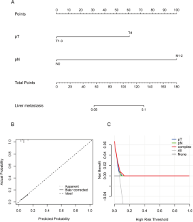
Data availability
The data that support the findings of this study are available from the corresponding author upon reasonable request.
Abbreviations
Rectal cancer
Carcinoembryonic antigen
Surveillance, Epidemiology, and End Results
American Joint Committee on Cancer
Overall survival
Computed tomography
Magnetic resonance imaging
Positron emission tomography-CT
Concordance-index
Decision curve analysis
Random survival forest
Confidence interval
Hazard ratio
Bray F, Laversanne M, Sung H, Ferlay J, Siegel RL, Soerjomataram I et al (2024) Global cancer statistics 2022: GLOBOCAN estimates of incidence and mortality worldwide for 36 cancers in 185 countries. CA Cancer J Clin 74:229–263
Article PubMed Google Scholar
van Gijn W, Marijnen CA, Nagtegaal ID, Kranenbarg EM, Putter H, Wiggers T et al (2011) Preoperative radiotherapy combined with total mesorectal excision for resectable rectal cancer: 12-year follow-up of the multicentre, randomised controlled TME trial. Lancet Oncol 12:575–582
Riihimaki M, Thomsen H, Sundquist K, Hemminki K (2012) Colorectal cancer patients: what do they die of? Frontline Gastroenterol 3:143–149
Article PubMed PubMed Central Google Scholar
Tjandra JJ, Chan MK (2007) Follow-up after curative resection of colorectal cancer: a meta-analysis. Dis Colon Rectum 50:1783–1799
Riihimaki M, Hemminki A, Sundquist J, Hemminki K (2016) Patterns of metastasis in colon and rectal cancer. Sci Rep 6:29765
Glynne-Jones R, Wyrwicz L, Tiret E, Brown G, Rodel C, Cervantes A et al (2017) Rectal cancer: ESMO clinical practice guidelines for diagnosis, treatment and follow-up. Ann Oncol 28:iv22–iv40
Article CAS PubMed Google Scholar
Benson AB, Venook AP, Adam M, Chang G, Chen YJ, Ciombor KK et al (2024) NCCN Guidelines® insights: rectal cancer, Version 3.2024. J Natl Compr Canc Netw 22:366–75
Ramphal W, Boeding JRE, van Iwaarden M, Schreinemakers JMJ, Rutten HJT, Crolla R et al (2019) Serum carcinoembryonic antigen to predict recurrence in the follow-up of patients with colorectal cancer. Int J Biol Markers 34:60–68
Sun Y, Deng Y, Xu M, Zhong J, Song J, Lin H et al (2023) A refined prediction of early recurrence combining tumor deposits in patients with resected rectal mucinous adenocarcinoma. Surg Today 53:762–772
Jiang D, Fan X, Chen K, Li H, Dai Y, Sun N et al (2023) Effects of magnetic resonance imaging (MRI)-detected extramural vascular invasion (mrEMVI) and tumor deposits (TDs) on distant metastasis and long-term survival after surgery for stage III rectal cancer: a retrospective study grouped based on the relationship between the bottom of the tumor and peritoneal reflection. J Gastrointest Oncol 14:963–979
Al-Sukhni E, Attwood K, Gabriel EM, LeVea CM, Kanehira K, Nurkin SJ (2017) Lymphovascular and perineural invasion are associated with poor prognostic features and outcomes in colorectal cancer: a retrospective cohort study. Int J Surg 37:42–49
Kobayashi H, Mochizuki H, Sugihara K, Morita T, Kotake K, Teramoto T et al (2007) Characteristics of recurrence and surveillance tools after curative resection for colorectal cancer: a multicenter study. Surgery 141:67–75
van Gestel YR, de Hingh IH, van Herk-Sukel MP, van Erning FN, Beerepoot LV, Wijsman JH et al (2014) Patterns of metachronous metastases after curative treatment of colorectal cancer. Cancer Epidemiol 38:448–454
Dienstmann R, Vermeulen L, Guinney J, Kopetz S, Tejpar S, Tabernero J (2017) Consensus molecular subtypes and the evolution of precision medicine in colorectal cancer. Nat Rev Cancer 17:79–92
Guinney J, Dienstmann R, Wang X, de Reynies A, Schlicker A, Soneson C et al (2015) The consensus molecular subtypes of colorectal cancer. Nat Med 21:1350–1356
Article CAS PubMed PubMed Central Google Scholar
Sveen A, Kopetz S, Lothe RA (2020) Biomarker-guided therapy for colorectal cancer: strength in complexity. Nat Rev Clin Oncol 17:11–32
Punt CJ, Koopman M, Vermeulen L (2017) From tumour heterogeneity to advances in precision treatment of colorectal cancer. Nat Rev Clin Oncol 14:235–246
Rodriguez-Salas N, Dominguez G, Barderas R, Mendiola M, García-Albéniz X, Maurel J et al (2017) Clinical relevance of colorectal cancer molecular subtypes. Crit Rev Oncol Hematol 109:9–19
Hanahan D, Weinberg RA (2011) Hallmarks of cancer: the next generation. Cell 144:646–674
Du LB, Li HZ, Wang YQ, Zhu C, Zheng RS, Zhang SW et al (2017) Report of colorectal cancer incidence and mortality in China, 2013. Zhonghua Zhong Liu Za Zhi 39:701–706
CAS PubMed Google Scholar
Manfredi S, Bouvier AM, Lepage C, Hatem C, Dancourt V, Faivre J (2006) Incidence and patterns of recurrence after resection for cure of colonic cancer in a well defined population. Br J Surg 93:1115–1122
Hackl C, Neumann P, Gerken M, Loss M, Klinkhammer-Schalke M, Schlitt HJ (2014) Treatment of colorectal liver metastases in Germany: a ten-year population-based analysis of 5772 cases of primary colorectal adenocarcinoma. BMC Cancer 14:810
Manfredi S, Lepage C, Hatem C, Coatmeur O, Faivre J, Bouvier AM (2006) Epidemiology and management of liver metastases from colorectal cancer. Ann Surg 244:254–259
Nordholm-Carstensen A, Krarup PM, Jorgensen LN, Wille-Jorgensen PA, Harling H, Danish Colorectal Cancer G (2014) Occurrence and survival of synchronous pulmonary metastases in colorectal cancer: a nationwide cohort study. Eur J Cancer 50:447–56
Ikoma N, You YN, Bednarski BK, Rodriguez-Bigas MA, Eng C, Das P et al (2017) Impact of recurrence and salvage surgery on survival after multidisciplinary treatment of rectal cancer. J Clin Oncol 35:2631–2638
Robinson JR, Newcomb PA, Hardikar S, Cohen SA, Phipps AI (2017) Stage IV colorectal cancer primary site and patterns of distant metastasis. Cancer Epidemiol 48:92–95
Qiu M, Hu J, Yang D, Cosgrove DP, Xu R (2015) Pattern of distant metastases in colorectal cancer: a SEER based study. Oncotarget 6:38658–38666
Tiselius C, Gunnarsson U, Smedh K, Glimelius B, Pahlman L (2013) Patients with rectal cancer receiving adjuvant chemotherapy have an increased survival: a population-based longitudinal study. Ann Oncol 24:160–165
Kirke R, Rajesh A, Verma R, Bankart MJ (2007) Rectal cancer: incidence of pulmonary metastases on thoracic CT and correlation with T staging. J Comput Assist Tomogr 31:569–571
Hogan J, O’Rourke C, Duff G, Burton M, Kelly N, Burke J et al (2014) Preoperative staging CT thorax in patients with colorectal cancer: its clinical importance. Dis Colon Rectum 57:1260–1266
Yongue G, Hotouras A, Murphy J, Mukhtar H, Bhan C, Chan CL (2015) The diagnostic yield of preoperative staging computed tomography of the thorax in colorectal cancer patients without hepatic metastases. Eur J Gastroenterol Hepatol 27:467–470
Nassar A, Aly NE, Jin Z, Aly EH (2024) ctDNA as a predictor of outcome after curative resection for locally advanced rectal cancer: systematic review and meta-analysis. Colorectal Dis 26:1346–1358
Tariq L, Arafah A, Sehar N, Ali A, Khan A, Rasool I et al (2023) Novel insights on perils and promises of miRNA in understanding colon cancer metastasis and progression. Med Oncol 40:282
Lin WC, Lin CC, Lin YY, Yang WH, Twu YC, Teng HW et al (2022) Molecular actions of exosomes and their theragnostics in colorectal cancer: current findings and limitations. Cell Oncol (Dordr) 45:1043–1052
Pan X, Yi X, Lan M, Su X, Zhou F, Wu W (2023) Research on the pathological mechanism of rectal adenocarcinoma based on DNA methylation. Medicine (Baltimore) 102:e32763
Leowattana W, Leowattana P, Leowattana T (2023) Systemic treatment for metastatic colorectal cancer. World J Gastroenterol 29:1569–1588
Seo SI, Lim SB, Yoon YS, Kim CW, Yu CS, Kim TW et al (2013) Comparison of recurrence patterns between </=5 years and >5 years after curative operations in colorectal cancer patients. J Surg Oncol 108:9–13
Cho YB, Chun HK, Yun HR, Lee WS, Yun SH, Lee WY (2007) Clinical and pathologic evaluation of patients with recurrence of colorectal cancer five or more years after curative resection. Dis Colon Rectum 50:1204–1210
Lee JL, Yu CS, Kim TW, Kim JH, Kim JC (2015) Rate of pulmonary metastasis varies with location of rectal cancer in the patients undergoing curative resection. World J Surg 39:759–768
Seo SI, Lim SB, Yoon YS, Kim CW, Yu CS, Kim TW et al (2013) Comparison of recurrence patterns between ≤5 years and >5 years after curative operations in colorectal cancer patients. J Surg Oncol 108:9–13
Download references
Acknowledgements
We thank all the investigators and patients who participated in the present study.
This work was supported by the Joint Funds for the National Clinical Key Specialty Construction Program (Grant No. 2021), the Fujian Provincial Clinical Research Center for Cancer Radiotherapy and Immunotherapy (Grant No. 2020Y2012), and Fujian Clinical Research Center for Radiation and Therapy of Digestive, Respiratory and Genitourinary Malignancies (Grant No. 2021Y2014).
Author information
Authors and affiliations.
Department of Radiation Oncology, Clinical Oncology School of Fujian Medical University, Fujian Cancer Hospital, Fuzhou, Fujian, China
Yilin Yu, Liang Hong, Jianjian Qiu, Shiji Wu, Lingdong Shao, Cheng Lin, Zhiping Wang & Junxin Wu
Shengli Clinical Medical College of Fujian Medical University, Fuzhou, Fujian, China
You can also search for this author in PubMed Google Scholar
Contributions
YY, JW, HW, ZW, CL, and LH designed this study. YY, HW, SW, JQ, and LS contributed to the data collection. YY, HW, and ZW analyzed the data. JW, CL, and LH supervised the study. YY, HW, and ZW wrote the manuscript. All authors read and approved the final manuscript.
Corresponding authors
Correspondence to Cheng Lin , Zhiping Wang or Junxin Wu .
Ethics declarations
Ethical approval and consent to participate.
The current study was approved by the ethics committee of Fujian Medical University Cancer Hospital, Fuzhou, China, and conducted in accordance with the principles of the Declaration of Helsinki and its amendment. All patients provided written informed consent prior to treatment, and all the information was anonymized prior to analysis.
Consent for publication
The manuscript has been approved by all authors for publication.
Competing interests
The authors declare no competing interests.
Additional information
Publisher's note.
Springer Nature remains neutral with regard to jurisdictional claims in published maps and institutional affiliations.
Yilin Yu, Haixia Wu, and Liang Hong contributed equally as first authors to this manuscript.
Supplementary Information
Below is the link to the electronic supplementary material.
Supplementary file1 (DOCX 52 KB)
Rights and permissions.
Springer Nature or its licensor (e.g. a society or other partner) holds exclusive rights to this article under a publishing agreement with the author(s) or other rightsholder(s); author self-archiving of the accepted manuscript version of this article is solely governed by the terms of such publishing agreement and applicable law.
Reprints and permissions
About this article
Yu, Y., Wu, H., Hong, L. et al. A large population-based and validated study on the follow-up management and supportive strategy of locally advanced rectal cancer patients. Support Care Cancer 32 , 652 (2024). https://doi.org/10.1007/s00520-024-08860-1
Download citation
Received : 07 March 2024
Accepted : 05 September 2024
Published : 11 September 2024
DOI : https://doi.org/10.1007/s00520-024-08860-1
Share this article
Anyone you share the following link with will be able to read this content:
Sorry, a shareable link is not currently available for this article.
Provided by the Springer Nature SharedIt content-sharing initiative
- Locally advanced rectal cancer
- Liver metastasis
- Lung metastasis
- Predictive model
- Follow-up strategy
- Find a journal
- Publish with us
- Track your research
COMMENTS
The t -test is frequently used in comparing 2 group means. The compared groups may be independent to each other such as men and women. Otherwise, compared data are correlated in a case such as comparison of blood pressure levels from the same person before and after medication (Figure 1). In this section we will focus on independent t -test only.
To test this, he recruits 20 subjects to participate in a study in which they each take the new drug for one month. He can perform a one sample t-test to determine if the mean reduction in blood pressure is significantly greater than the mean reduction that results from the current standard drug. Examples: Independent Two Sample t-tests in Real ...
Issues of Concern. Selecting appropriate statistical tests is a critical step in conducting research. [2] Therefore, there are 3 forms of Student's t-test about which physicians, particularly physician-scientists, need to be aware: (1) 1-sample t-test, (2) 2-sample t-test, and (3) 2-sample paired t-test. The 1-sample t-test evaluates a single ...
Independent Samples T Tests Hypotheses. Independent samples t tests have the following hypotheses: Null hypothesis: The means for the two populations are equal. Alternative hypothesis: The means for the two populations are not equal.; If the p-value is less than your significance level (e.g., 0.05), you can reject the null hypothesis. The difference between the two means is statistically ...
for a study to find a certain effect with sufficient power. In the next section, we explain how such sample-size calculation can be performed for the two-sample t test. 1 In this article, we focus on sample-size calculations in which the effect (i.e., difference in means) and the vari-ance of the data are separately defined as opposed to
In medical research, various t -tests and Chi-square tests are the two types of statistical tests most commonly used. In any statistical hypothesis testing situation, if the test statistic follows a Student's t -test distribution under null hypothesis, it is a t -test. Most frequently used t -tests are: For comparison of mean in single sample ...
An Independent T-test or Independent Samples T-test is an important test for Between Groups differences.. Here we will discuss the underlying assumptions of the Independent t-test and explain how to interpret the results of the t-test. There are a number of assumptions that need to be met before performing an Independent t-test:
We'll use a two-sample t test to evaluate if the difference between the two group means is statistically significant. The t test output is below. In the output, you can see that the treatment group (Sample 1) has a mean of 109 while the control group's (Sample 2) average is 100. The p-value for the difference between the groups is 0.112.
When to use a t test. A t test can only be used when comparing the means of two groups (a.k.a. pairwise comparison). If you want to compare more than two groups, or if you want to do multiple pairwise comparisons, use an ANOVA test or a post-hoc test.. The t test is a parametric test of difference, meaning that it makes the same assumptions about your data as other parametric tests.
Reporting the result of an independent t-test. When reporting the result of an independent t-test, you need to include the t-statistic value, the degrees of freedom (df) and the significance value of the test (p-value).The format of the test result is: t(df) = t-statistic, p = significance value. Therefore, for the example above, you could report the result as t(7.001) = 2.233, p = 0.061.
The Independent Samples t Test is commonly used to test the following: Statistical differences between the means of two groups. Statistical differences between the means of two interventions. Statistical differences between the means of two change scores. Note: The Independent Samples t Test can only compare the means for two (and only two) groups.
The independent samples t-test compares two independent groups of observations or measurements on a single characteristic. The independent samples t-test is the between-subjects analog to the dependent samples t-test, which is used when the study involves a repeated measurement (e.g., pretest vs. posttest) or matched observations (e.g., older ...
The research question I'm interested in is whether Anastasia or Bernadette is a better tutor, or if it doesn't make much of a difference. ... Not surprisingly, you can run an independent samples t-test using the t.test() function (Section 13.7), but once again I'm going to start with a somewhat simpler function in the lsr package.
The research question I'm interested in is whether Anastasia or Bernadette is a better tutor, or if it doesn't make much of a difference. ... Not surprisingly, you can run an independent samples t-test using the t.test() function (Section 13.7), but once again I'm going to start with a somewhat simpler function in the lsr package.
two groups. The independent t- test depends on the means, standard deviation s and sample sizes. of each group. Various assumptions also need to be made - see validity section below. The ...
Student's t test (t test), analysis of variance (ANOVA), and analysis of covariance (ANCOVA) are statistical methods used in the testing of hypothesis for comparison of means between the groups.The Student's t test is used to compare the means between two groups, whereas ANOVA is used to compare the means among three or more groups. In ANOVA, first gets a common P value.
Note: If you have more than 2 treatment groups in your study (e.g., 3 groups: diet, exercise and drug treatment groups), but only wanted to compared two (e.g., the diet and drug treatment groups), you could type in 1 to Group 1: box and 3 to Group 2: box (i.e., if you wished to compare the diet with drug treatment). Click the button.; If you need to change the confidence level limits or change ...
In the next section we explain why you are using an independent-samples t-test to analyse your results, rather than simply using descriptive statistics.. SPSS Statistics Understanding why the independent-samples t-test is being used. To briefly recap, an independent-samples t-test is used to determine whether there is a difference between two independent, unrelated groups (e.g., undergraduate ...
t(degrees of freedom) = the t statistic, p = p value. An independent-samples t-test was run to determine if the Mind Over Matter coping strategy was more effective at reducing anxiety than deep breathing exercises. The results showed that the participants using the Mind Over Matter strategy (M = 21, SD = 2.2) reported lower levels of anxiety ...
An independent samples t-test compares the means of two groups. The data are interval for the groups. There is not an assumption of normal distribution (if the distribution of one or both groups is really unusual, the t-test will not give good results with unequal sample sizes), but there is an assumption that the two standard deviations are equal. . If the sample sizes are equal or very ...
8. Use a table of critical t-values (see the one at the back of this document) The critical t-value at the p = .05 significance level, for a two-tailed test, is: 2.262. Our t-value (from the experiment) was: 2.183. In order for this to be significant, it must be LARGER than the critical t-value derived from the table.
Note: The "M" in the results stands for sample mean, the "SD" stands for sample standard deviation, and "df" stands for degrees of freedom associated with the t-test statistic. The following examples show how to report the results of each type of t-test in practice. Example: Reporting Results of a One Sample T-Test. A botanist wants ...
In this study, the results were analyzed using Student's t-test [31] of an independent two-sample t-test, which was used to compare the mean scores between the two groups. The null hypothesis was ...
The paired t-test is a straight-forward extension of the independent sample t-test; the key concept is that the two samples are no longer independent, they are paired. Thus, instead of mean of group 1 minus mean of group two, we test the differences between sample 1 and sample 2 for each paired observation.
Collectively, these studies showed that 1) IL-4 has a direct impact on CART cells that is independent of the presence of tumor cells, 2) IL-4 supplementation drives CART cell exhaustion in various ...
In the study, none of the patients (0/30) considered low-risk by the DecisionDx-Melanoma test (less than 5% predicted risk of SLN positivity) had a positive SLN, compared to a 31.9% SLN positivity ...
The dependent t-test can be used to test either a "change" or a "difference" in means between two related groups, but not both at the same time. Whether you are measuring a "change" or "difference" between the means of the two related groups depends on your study design.
A t test is also known as Student's t test. It is a statistical analysis technique that was developed by William Sealy Gosset in 1908 as a means to control the quality of dark beers. A t test used to test whether there is a difference between two independent sample means is not different from a t test used when there is only one sample (as ...
Background Chewing gum is a healthy, cheap, and familiar solution for patients with premature irritation of the stomach and intestines. This study compared the effect of chewing gum and the routine method on ileus after burns. Methods This study is a randomized clinical trial conducted in Valiasr Hospital in Arak, Markazi Province, in the center of Iran, from December 2021 to February 2023 ...
Objective Our objective was to evaluate the predictive factors and metastatic time for liver and lung metastasis in locally advanced rectal cancer (RC) patients. Methods Univariate and multivariate analysis were performed to identify risk factors and prognostic factors for liver metastasis and lung metastasis in RC. Survival probabilities were calculated using the Kaplan-Meier model and ...