- Skip to secondary menu
- Skip to main content
- Skip to primary sidebar
Statistics By Jim
Making statistics intuitive

Statistical Hypothesis Testing Overview
By Jim Frost 59 Comments
In this blog post, I explain why you need to use statistical hypothesis testing and help you navigate the essential terminology. Hypothesis testing is a crucial procedure to perform when you want to make inferences about a population using a random sample. These inferences include estimating population properties such as the mean, differences between means, proportions, and the relationships between variables.
This post provides an overview of statistical hypothesis testing. If you need to perform hypothesis tests, consider getting my book, Hypothesis Testing: An Intuitive Guide .
Why You Should Perform Statistical Hypothesis Testing

Hypothesis testing is a form of inferential statistics that allows us to draw conclusions about an entire population based on a representative sample. You gain tremendous benefits by working with a sample. In most cases, it is simply impossible to observe the entire population to understand its properties. The only alternative is to collect a random sample and then use statistics to analyze it.
While samples are much more practical and less expensive to work with, there are trade-offs. When you estimate the properties of a population from a sample, the sample statistics are unlikely to equal the actual population value exactly. For instance, your sample mean is unlikely to equal the population mean. The difference between the sample statistic and the population value is the sample error.
Differences that researchers observe in samples might be due to sampling error rather than representing a true effect at the population level. If sampling error causes the observed difference, the next time someone performs the same experiment the results might be different. Hypothesis testing incorporates estimates of the sampling error to help you make the correct decision. Learn more about Sampling Error .
For example, if you are studying the proportion of defects produced by two manufacturing methods, any difference you observe between the two sample proportions might be sample error rather than a true difference. If the difference does not exist at the population level, you won’t obtain the benefits that you expect based on the sample statistics. That can be a costly mistake!
Let’s cover some basic hypothesis testing terms that you need to know.
Background information : Difference between Descriptive and Inferential Statistics and Populations, Parameters, and Samples in Inferential Statistics
Hypothesis Testing
Hypothesis testing is a statistical analysis that uses sample data to assess two mutually exclusive theories about the properties of a population. Statisticians call these theories the null hypothesis and the alternative hypothesis. A hypothesis test assesses your sample statistic and factors in an estimate of the sample error to determine which hypothesis the data support.
When you can reject the null hypothesis, the results are statistically significant, and your data support the theory that an effect exists at the population level.
The effect is the difference between the population value and the null hypothesis value. The effect is also known as population effect or the difference. For example, the mean difference between the health outcome for a treatment group and a control group is the effect.
Typically, you do not know the size of the actual effect. However, you can use a hypothesis test to help you determine whether an effect exists and to estimate its size. Hypothesis tests convert your sample effect into a test statistic, which it evaluates for statistical significance. Learn more about Test Statistics .
An effect can be statistically significant, but that doesn’t necessarily indicate that it is important in a real-world, practical sense. For more information, read my post about Statistical vs. Practical Significance .
Null Hypothesis
The null hypothesis is one of two mutually exclusive theories about the properties of the population in hypothesis testing. Typically, the null hypothesis states that there is no effect (i.e., the effect size equals zero). The null is often signified by H 0 .
In all hypothesis testing, the researchers are testing an effect of some sort. The effect can be the effectiveness of a new vaccination, the durability of a new product, the proportion of defect in a manufacturing process, and so on. There is some benefit or difference that the researchers hope to identify.
However, it’s possible that there is no effect or no difference between the experimental groups. In statistics, we call this lack of an effect the null hypothesis. Therefore, if you can reject the null, you can favor the alternative hypothesis, which states that the effect exists (doesn’t equal zero) at the population level.
You can think of the null as the default theory that requires sufficiently strong evidence against in order to reject it.
For example, in a 2-sample t-test, the null often states that the difference between the two means equals zero.
When you can reject the null hypothesis, your results are statistically significant. Learn more about Statistical Significance: Definition & Meaning .
Related post : Understanding the Null Hypothesis in More Detail
Alternative Hypothesis
The alternative hypothesis is the other theory about the properties of the population in hypothesis testing. Typically, the alternative hypothesis states that a population parameter does not equal the null hypothesis value. In other words, there is a non-zero effect. If your sample contains sufficient evidence, you can reject the null and favor the alternative hypothesis. The alternative is often identified with H 1 or H A .
For example, in a 2-sample t-test, the alternative often states that the difference between the two means does not equal zero.
You can specify either a one- or two-tailed alternative hypothesis:
If you perform a two-tailed hypothesis test, the alternative states that the population parameter does not equal the null value. For example, when the alternative hypothesis is H A : μ ≠ 0, the test can detect differences both greater than and less than the null value.
A one-tailed alternative has more power to detect an effect but it can test for a difference in only one direction. For example, H A : μ > 0 can only test for differences that are greater than zero.
Related posts : Understanding T-tests and One-Tailed and Two-Tailed Hypothesis Tests Explained

P-values are the probability that you would obtain the effect observed in your sample, or larger, if the null hypothesis is correct. In simpler terms, p-values tell you how strongly your sample data contradict the null. Lower p-values represent stronger evidence against the null. You use P-values in conjunction with the significance level to determine whether your data favor the null or alternative hypothesis.
Related post : Interpreting P-values Correctly
Significance Level (Alpha)

For instance, a significance level of 0.05 signifies a 5% risk of deciding that an effect exists when it does not exist.
Use p-values and significance levels together to help you determine which hypothesis the data support. If the p-value is less than your significance level, you can reject the null and conclude that the effect is statistically significant. In other words, the evidence in your sample is strong enough to be able to reject the null hypothesis at the population level.
Related posts : Graphical Approach to Significance Levels and P-values and Conceptual Approach to Understanding Significance Levels
Types of Errors in Hypothesis Testing
Statistical hypothesis tests are not 100% accurate because they use a random sample to draw conclusions about entire populations. There are two types of errors related to drawing an incorrect conclusion.
- False positives: You reject a null that is true. Statisticians call this a Type I error . The Type I error rate equals your significance level or alpha (α).
- False negatives: You fail to reject a null that is false. Statisticians call this a Type II error. Generally, you do not know the Type II error rate. However, it is a larger risk when you have a small sample size , noisy data, or a small effect size. The type II error rate is also known as beta (β).
Statistical power is the probability that a hypothesis test correctly infers that a sample effect exists in the population. In other words, the test correctly rejects a false null hypothesis. Consequently, power is inversely related to a Type II error. Power = 1 – β. Learn more about Power in Statistics .
Related posts : Types of Errors in Hypothesis Testing and Estimating a Good Sample Size for Your Study Using Power Analysis
Which Type of Hypothesis Test is Right for You?
There are many different types of procedures you can use. The correct choice depends on your research goals and the data you collect. Do you need to understand the mean or the differences between means? Or, perhaps you need to assess proportions. You can even use hypothesis testing to determine whether the relationships between variables are statistically significant.
To choose the proper statistical procedure, you’ll need to assess your study objectives and collect the correct type of data . This background research is necessary before you begin a study.
Related Post : Hypothesis Tests for Continuous, Binary, and Count Data
Statistical tests are crucial when you want to use sample data to make conclusions about a population because these tests account for sample error. Using significance levels and p-values to determine when to reject the null hypothesis improves the probability that you will draw the correct conclusion.
To see an alternative approach to these traditional hypothesis testing methods, learn about bootstrapping in statistics !
If you want to see examples of hypothesis testing in action, I recommend the following posts that I have written:
- How Effective Are Flu Shots? This example shows how you can use statistics to test proportions.
- Fatality Rates in Star Trek . This example shows how to use hypothesis testing with categorical data.
- Busting Myths About the Battle of the Sexes . A fun example based on a Mythbusters episode that assess continuous data using several different tests.
- Are Yawns Contagious? Another fun example inspired by a Mythbusters episode.
Share this:

Reader Interactions

January 14, 2024 at 8:43 am
Hello professor Jim, how are you doing! Pls. What are the properties of a population and their examples? Thanks for your time and understanding.

January 14, 2024 at 12:57 pm
Please read my post about Populations vs. Samples for more information and examples.
Also, please note there is a search bar in the upper-right margin of my website. Use that to search for topics.

July 5, 2023 at 7:05 am
Hello, I have a question as I read your post. You say in p-values section
“P-values are the probability that you would obtain the effect observed in your sample, or larger, if the null hypothesis is correct. In simpler terms, p-values tell you how strongly your sample data contradict the null. Lower p-values represent stronger evidence against the null.”
But according to your definition of effect, the null states that an effect does not exist, correct? So what I assume you want to say is that “P-values are the probability that you would obtain the effect observed in your sample, or larger, if the null hypothesis is **incorrect**.”
July 6, 2023 at 5:18 am
Hi Shrinivas,
The correct definition of p-value is that it is a probability that exists in the context of a true null hypothesis. So, the quotation is correct in stating “if the null hypothesis is correct.”
Essentially, the p-value tells you the likelihood of your observed results (or more extreme) if the null hypothesis is true. It gives you an idea of whether your results are surprising or unusual if there is no effect.
Hence, with sufficiently low p-values, you reject the null hypothesis because it’s telling you that your sample results were unlikely to have occurred if there was no effect in the population.
I hope that helps make it more clear. If not, let me know I’ll attempt to clarify!

May 8, 2023 at 12:47 am
Thanks a lot Ny best regards
May 7, 2023 at 11:15 pm
Hi Jim Can you tell me something about size effect? Thanks
May 8, 2023 at 12:29 am
Here’s a post that I’ve written about Effect Sizes that will hopefully tell you what you need to know. Please read that. Then, if you have any more specific questions about effect sizes, please post them there. Thanks!

January 7, 2023 at 4:19 pm
Hi Jim, I have only read two pages so far but I am really amazed because in few paragraphs you made me clearly understand the concepts of months of courses I received in biostatistics! Thanks so much for this work you have done it helps a lot!
January 10, 2023 at 3:25 pm
Thanks so much!

June 17, 2021 at 1:45 pm
Can you help in the following question: Rocinante36 is priced at ₹7 lakh and has been designed to deliver a mileage of 22 km/litre and a top speed of 140 km/hr. Formulate the null and alternative hypotheses for mileage and top speed to check whether the new models are performing as per the desired design specifications.

April 19, 2021 at 1:51 pm
Its indeed great to read your work statistics.
I have a doubt regarding the one sample t-test. So as per your book on hypothesis testing with reference to page no 45, you have mentioned the difference between “the sample mean and the hypothesised mean is statistically significant”. So as per my understanding it should be quoted like “the difference between the population mean and the hypothesised mean is statistically significant”. The catch here is the hypothesised mean represents the sample mean.
Please help me understand this.
Regards Rajat
April 19, 2021 at 3:46 pm
Thanks for buying my book. I’m so glad it’s been helpful!
The test is performed on the sample but the results apply to the population. Hence, if the difference between the sample mean (observed in your study) and the hypothesized mean is statistically significant, that suggests that population does not equal the hypothesized mean.
For one sample tests, the hypothesized mean is not the sample mean. It is a mean that you want to use for the test value. It usually represents a value that is important to your research. In other words, it’s a value that you pick for some theoretical/practical reasons. You pick it because you want to determine whether the population mean is different from that particular value.
I hope that helps!

November 5, 2020 at 6:24 am
Jim, you are such a magnificent statistician/economist/econometrician/data scientist etc whatever profession. Your work inspires and simplifies the lives of so many researchers around the world. I truly admire you and your work. I will buy a copy of each book you have on statistics or econometrics. Keep doing the good work. Remain ever blessed
November 6, 2020 at 9:47 pm
Hi Renatus,
Thanks so much for you very kind comments. You made my day!! I’m so glad that my website has been helpful. And, thanks so much for supporting my books! 🙂

November 2, 2020 at 9:32 pm
Hi Jim, I hope you are aware of 2019 American Statistical Association’s official statement on Statistical Significance: https://www.tandfonline.com/doi/full/10.1080/00031305.2019.1583913 In case you do not bother reading the full article, may I quote you the core message here: “We conclude, based on our review of the articles in this special issue and the broader literature, that it is time to stop using the term “statistically significant” entirely. Nor should variants such as “significantly different,” “p < 0.05,” and “nonsignificant” survive, whether expressed in words, by asterisks in a table, or in some other way."
With best wishes,
November 3, 2020 at 2:09 am
I’m definitely aware of the debate surrounding how to use p-values most effectively. However, I need to correct you on one point. The link you provide is NOT a statement by the American Statistical Association. It is an editorial by several authors.
There is considerable debate over this issue. There are problems with p-values. However, as the authors state themselves, much of the problem is over people’s mindsets about how to use p-values and their incorrect interpretations about what statistical significance does and does not mean.
If you were to read my website more thoroughly, you’d be aware that I share many of their concerns and I address them in multiple posts. One of the authors’ key points is the need to be thoughtful and conduct thoughtful research and analysis. I emphasize this aspect in multiple posts on this topic. I’ll ask you to read the following three because they all address some of the authors’ concerns and suggestions. But you might run across others to read as well.
Five Tips for Using P-values to Avoid Being Misled How to Interpret P-values Correctly P-values and the Reproducibility of Experimental Results

September 24, 2020 at 11:52 pm
HI Jim, i just want you to know that you made explanation for Statistics so simple! I should say lesser and fewer words that reduce the complexity. All the best! 🙂
September 25, 2020 at 1:03 am
Thanks, Rene! Your kind words mean a lot to me! I’m so glad it has been helpful!

September 23, 2020 at 2:21 am
Honestly, I never understood stats during my entire M.Ed course and was another nightmare for me. But how easily you have explained each concept, I have understood stats way beyond my imagination. Thank you so much for helping ignorant research scholars like us. Looking forward to get hardcopy of your book. Kindly tell is it available through flipkart?
September 24, 2020 at 11:14 pm
I’m so happy to hear that my website has been helpful!
I checked on flipkart and it appears like my books are not available there. I’m never exactly sure where they’re available due to the vagaries of different distribution channels. They are available on Amazon in India.
Introduction to Statistics: An Intuitive Guide (Amazon IN) Hypothesis Testing: An Intuitive Guide (Amazon IN)

July 26, 2020 at 11:57 am
Dear Jim I am a teacher from India . I don’t have any background in statistics, and still I should tell that in a single read I can follow your explanations . I take my entire biostatistics class for botany graduates with your explanations. Thanks a lot. May I know how I can avail your books in India
July 28, 2020 at 12:31 am
Right now my books are only available as ebooks from my website. However, soon I’ll have some exciting news about other ways to obtain it. Stay tuned! I’ll announce it on my email list. If you’re not already on it, you can sign up using the form that is in the right margin of my website.

June 22, 2020 at 2:02 pm
Also can you please let me if this book covers topics like EDA and principal component analysis?
June 22, 2020 at 2:07 pm
This book doesn’t cover principal components analysis. Although, I wouldn’t really classify that as a hypothesis test. In the future, I might write a multivariate analysis book that would cover this and others. But, that’s well down the road.
My Introduction to Statistics covers EDA. That’s the largely graphical look at your data that you often do prior to hypothesis testing. The Introduction book perfectly leads right into the Hypothesis Testing book.
June 22, 2020 at 1:45 pm
Thanks for the detailed explanation. It does clear my doubts. I saw that your book related to hypothesis testing has the topics that I am studying currently. I am looking forward to purchasing it.
Regards, Take Care
June 19, 2020 at 1:03 pm
For this particular article I did not understand a couple of statements and it would great if you could help: 1)”If sample error causes the observed difference, the next time someone performs the same experiment the results might be different.” 2)”If the difference does not exist at the population level, you won’t obtain the benefits that you expect based on the sample statistics.”
I discovered your articles by chance and now I keep coming back to read & understand statistical concepts. These articles are very informative & easy to digest. Thanks for the simplifying things.
June 20, 2020 at 9:53 pm
I’m so happy to hear that you’ve found my website to be helpful!
To answer your questions, keep in mind that a central tenant of inferential statistics is that the random sample that a study drew was only one of an infinite number of possible it could’ve drawn. Each random sample produces different results. Most results will cluster around the population value assuming they used good methodology. However, random sampling error always exists and makes it so that population estimates from a sample almost never exactly equal the correct population value.
So, imagine that we’re studying a medication and comparing the treatment and control groups. Suppose that the medicine is truly not effect and that the population difference between the treatment and control group is zero (i.e., no difference.) Despite the true difference being zero, most sample estimates will show some degree of either a positive or negative effect thanks to random sampling error. So, just because a study has an observed difference does not mean that a difference exists at the population level. So, on to your questions:
1. If the observed difference is just random error, then it makes sense that if you collected another random sample, the difference could change. It could change from negative to positive, positive to negative, more extreme, less extreme, etc. However, if the difference exists at the population level, most random samples drawn from the population will reflect that difference. If the medicine has an effect, most random samples will reflect that fact and not bounce around on both sides of zero as much.
2. This is closely related to the previous answer. If there is no difference at the population level, but say you approve the medicine because of the observed effects in a sample. Even though your random sample showed an effect (which was really random error), that effect doesn’t exist. So, when you start using it on a larger scale, people won’t benefit from the medicine. That’s why it’s important to separate out what is easily explained by random error versus what is not easily explained by it.
I think reading my post about how hypothesis tests work will help clarify this process. Also, in about 24 hours (as I write this), I’ll be releasing my new ebook about Hypothesis Testing!

May 29, 2020 at 5:23 am
Hi Jim, I really enjoy your blog. Can you please link me on your blog where you discuss about Subgroup analysis and how it is done? I need to use non parametric and parametric statistical methods for my work and also do subgroup analysis in order to identify potential groups of patients that may benefit more from using a treatment than other groups.
May 29, 2020 at 2:12 pm
Hi, I don’t have a specific article about subgroup analysis. However, subgroup analysis is just the dividing up of a larger sample into subgroups and then analyzing those subgroups separately. You can use the various analyses I write about on the subgroups.
Alternatively, you can include the subgroups in regression analysis as an indicator variable and include that variable as a main effect and an interaction effect to see how the relationships vary by subgroup without needing to subdivide your data. I write about that approach in my article about comparing regression lines . This approach is my preferred approach when possible.

April 19, 2020 at 7:58 am
sir is confidence interval is a part of estimation?

April 17, 2020 at 3:36 pm
Sir can u plz briefly explain alternatives of hypothesis testing? I m unable to find the answer
April 18, 2020 at 1:22 am
Assuming you want to draw conclusions about populations by using samples (i.e., inferential statistics ), you can use confidence intervals and bootstrap methods as alternatives to the traditional hypothesis testing methods.

March 9, 2020 at 10:01 pm
Hi JIm, could you please help with activities that can best teach concepts of hypothesis testing through simulation, Also, do you have any question set that would enhance students intuition why learning hypothesis testing as a topic in introductory statistics. Thanks.

March 5, 2020 at 3:48 pm
Hi Jim, I’m studying multiple hypothesis testing & was wondering if you had any material that would be relevant. I’m more trying to understand how testing multiple samples simultaneously affects your results & more on the Bonferroni Correction
March 5, 2020 at 4:05 pm
I write about multiple comparisons (aka post hoc tests) in the ANOVA context . I don’t talk about Bonferroni Corrections specifically but I cover related types of corrections. I’m not sure if that exactly addresses what you want to know but is probably the closest I have already written. I hope it helps!

January 14, 2020 at 9:03 pm
Thank you! Have a great day/evening.
January 13, 2020 at 7:10 pm
Any help would be greatly appreciated. What is the difference between The Hypothesis Test and The Statistical Test of Hypothesis?
January 14, 2020 at 11:02 am
They sound like the same thing to me. Unless this is specialized terminology for a particular field or the author was intending something specific, I’d guess they’re one and the same.

April 1, 2019 at 10:00 am
so these are the only two forms of Hypothesis used in statistical testing?
April 1, 2019 at 10:02 am
Are you referring to the null and alternative hypothesis? If so, yes, that’s those are the standard hypotheses in a statistical hypothesis test.
April 1, 2019 at 9:57 am
year very insightful post, thanks for the write up

October 27, 2018 at 11:09 pm
hi there, am upcoming statistician, out of all blogs that i have read, i have found this one more useful as long as my problem is concerned. thanks so much
October 27, 2018 at 11:14 pm
Hi Stano, you’re very welcome! Thanks for your kind words. They mean a lot! I’m happy to hear that my posts were able to help you. I’m sure you will be a fantastic statistician. Best of luck with your studies!

October 26, 2018 at 11:39 am
Dear Jim, thank you very much for your explanations! I have a question. Can I use t-test to compare two samples in case each of them have right bias?
October 26, 2018 at 12:00 pm
Hi Tetyana,
You’re very welcome!
The term “right bias” is not a standard term. Do you by chance mean right skewed distributions? In other words, if you plot the distribution for each group on a histogram they have longer right tails? These are not the symmetrical bell-shape curves of the normal distribution.
If that’s the case, yes you can as long as you exceed a specific sample size within each group. I include a table that contains these sample size requirements in my post about nonparametric vs parametric analyses .
Bias in statistics refers to cases where an estimate of a value is systematically higher or lower than the true value. If this is the case, you might be able to use t-tests, but you’d need to be sure to understand the nature of the bias so you would understand what the results are really indicating.
I hope this helps!

April 2, 2018 at 7:28 am
Simple and upto the point 👍 Thank you so much.
April 2, 2018 at 11:11 am
Hi Kalpana, thanks! And I’m glad it was helpful!

March 26, 2018 at 8:41 am
Am I correct if I say: Alpha – Probability of wrongly rejection of null hypothesis P-value – Probability of wrongly acceptance of null hypothesis
March 28, 2018 at 3:14 pm
You’re correct about alpha. Alpha is the probability of rejecting the null hypothesis when the null is true.
Unfortunately, your definition of the p-value is a bit off. The p-value has a fairly convoluted definition. It is the probability of obtaining the effect observed in a sample, or more extreme, if the null hypothesis is true. The p-value does NOT indicate the probability that either the null or alternative is true or false. Although, those are very common misinterpretations. To learn more, read my post about how to interpret p-values correctly .

March 2, 2018 at 6:10 pm
I recently started reading your blog and it is very helpful to understand each concept of statistical tests in easy way with some good examples. Also, I recommend to other people go through all these blogs which you posted. Specially for those people who have not statistical background and they are facing to many problems while studying statistical analysis.
Thank you for your such good blogs.
March 3, 2018 at 10:12 pm
Hi Amit, I’m so glad that my blog posts have been helpful for you! It means a lot to me that you took the time to write such a nice comment! Also, thanks for recommending by blog to others! I try really hard to write posts about statistics that are easy to understand.

January 17, 2018 at 7:03 am
I recently started reading your blog and I find it very interesting. I am learning statistics by my own, and I generally do many google search to understand the concepts. So this blog is quite helpful for me, as it have most of the content which I am looking for.
January 17, 2018 at 3:56 pm
Hi Shashank, thank you! And, I’m very glad to hear that my blog is helpful!

January 2, 2018 at 2:28 pm
thank u very much sir.
January 2, 2018 at 2:36 pm
You’re very welcome, Hiral!

November 21, 2017 at 12:43 pm
Thank u so much sir….your posts always helps me to be a #statistician
November 21, 2017 at 2:40 pm
Hi Sachin, you’re very welcome! I’m happy that you find my posts to be helpful!

November 19, 2017 at 8:22 pm
great post as usual, but it would be nice to see an example.
November 19, 2017 at 8:27 pm
Thank you! At the end of this post, I have links to four other posts that show examples of hypothesis tests in action. You’ll find what you’re looking for in those posts!
Comments and Questions Cancel reply
Reset password New user? Sign up
Existing user? Log in
Hypothesis Testing
Already have an account? Log in here.
A hypothesis test is a statistical inference method used to test the significance of a proposed (hypothesized) relation between population statistics (parameters) and their corresponding sample estimators . In other words, hypothesis tests are used to determine if there is enough evidence in a sample to prove a hypothesis true for the entire population.
The test considers two hypotheses: the null hypothesis , which is a statement meant to be tested, usually something like "there is no effect" with the intention of proving this false, and the alternate hypothesis , which is the statement meant to stand after the test is performed. The two hypotheses must be mutually exclusive ; moreover, in most applications, the two are complementary (one being the negation of the other). The test works by comparing the \(p\)-value to the level of significance (a chosen target). If the \(p\)-value is less than or equal to the level of significance, then the null hypothesis is rejected.
When analyzing data, only samples of a certain size might be manageable as efficient computations. In some situations the error terms follow a continuous or infinite distribution, hence the use of samples to suggest accuracy of the chosen test statistics. The method of hypothesis testing gives an advantage over guessing what distribution or which parameters the data follows.
Definitions and Methodology
Hypothesis test and confidence intervals.
In statistical inference, properties (parameters) of a population are analyzed by sampling data sets. Given assumptions on the distribution, i.e. a statistical model of the data, certain hypotheses can be deduced from the known behavior of the model. These hypotheses must be tested against sampled data from the population.
The null hypothesis \((\)denoted \(H_0)\) is a statement that is assumed to be true. If the null hypothesis is rejected, then there is enough evidence (statistical significance) to accept the alternate hypothesis \((\)denoted \(H_1).\) Before doing any test for significance, both hypotheses must be clearly stated and non-conflictive, i.e. mutually exclusive, statements. Rejecting the null hypothesis, given that it is true, is called a type I error and it is denoted \(\alpha\), which is also its probability of occurrence. Failing to reject the null hypothesis, given that it is false, is called a type II error and it is denoted \(\beta\), which is also its probability of occurrence. Also, \(\alpha\) is known as the significance level , and \(1-\beta\) is known as the power of the test. \(H_0\) \(\textbf{is true}\)\(\hspace{15mm}\) \(H_0\) \(\textbf{is false}\) \(\textbf{Reject}\) \(H_0\)\(\hspace{10mm}\) Type I error Correct Decision \(\textbf{Reject}\) \(H_1\) Correct Decision Type II error The test statistic is the standardized value following the sampled data under the assumption that the null hypothesis is true, and a chosen particular test. These tests depend on the statistic to be studied and the assumed distribution it follows, e.g. the population mean following a normal distribution. The \(p\)-value is the probability of observing an extreme test statistic in the direction of the alternate hypothesis, given that the null hypothesis is true. The critical value is the value of the assumed distribution of the test statistic such that the probability of making a type I error is small.
Methodologies: Given an estimator \(\hat \theta\) of a population statistic \(\theta\), following a probability distribution \(P(T)\), computed from a sample \(\mathcal{S},\) and given a significance level \(\alpha\) and test statistic \(t^*,\) define \(H_0\) and \(H_1;\) compute the test statistic \(t^*.\) \(p\)-value Approach (most prevalent): Find the \(p\)-value using \(t^*\) (right-tailed). If the \(p\)-value is at most \(\alpha,\) reject \(H_0\). Otherwise, reject \(H_1\). Critical Value Approach: Find the critical value solving the equation \(P(T\geq t_\alpha)=\alpha\) (right-tailed). If \(t^*>t_\alpha\), reject \(H_0\). Otherwise, reject \(H_1\). Note: Failing to reject \(H_0\) only means inability to accept \(H_1\), and it does not mean to accept \(H_0\).
Assume a normally distributed population has recorded cholesterol levels with various statistics computed. From a sample of 100 subjects in the population, the sample mean was 214.12 mg/dL (milligrams per deciliter), with a sample standard deviation of 45.71 mg/dL. Perform a hypothesis test, with significance level 0.05, to test if there is enough evidence to conclude that the population mean is larger than 200 mg/dL. Hypothesis Test We will perform a hypothesis test using the \(p\)-value approach with significance level \(\alpha=0.05:\) Define \(H_0\): \(\mu=200\). Define \(H_1\): \(\mu>200\). Since our values are normally distributed, the test statistic is \(z^*=\frac{\bar X - \mu_0}{\frac{s}{\sqrt{n}}}=\frac{214.12 - 200}{\frac{45.71}{\sqrt{100}}}\approx 3.09\). Using a standard normal distribution, we find that our \(p\)-value is approximately \(0.001\). Since the \(p\)-value is at most \(\alpha=0.05,\) we reject \(H_0\). Therefore, we can conclude that the test shows sufficient evidence to support the claim that \(\mu\) is larger than \(200\) mg/dL.
If the sample size was smaller, the normal and \(t\)-distributions behave differently. Also, the question itself must be managed by a double-tail test instead.
Assume a population's cholesterol levels are recorded and various statistics are computed. From a sample of 25 subjects, the sample mean was 214.12 mg/dL (milligrams per deciliter), with a sample standard deviation of 45.71 mg/dL. Perform a hypothesis test, with significance level 0.05, to test if there is enough evidence to conclude that the population mean is not equal to 200 mg/dL. Hypothesis Test We will perform a hypothesis test using the \(p\)-value approach with significance level \(\alpha=0.05\) and the \(t\)-distribution with 24 degrees of freedom: Define \(H_0\): \(\mu=200\). Define \(H_1\): \(\mu\neq 200\). Using the \(t\)-distribution, the test statistic is \(t^*=\frac{\bar X - \mu_0}{\frac{s}{\sqrt{n}}}=\frac{214.12 - 200}{\frac{45.71}{\sqrt{25}}}\approx 1.54\). Using a \(t\)-distribution with 24 degrees of freedom, we find that our \(p\)-value is approximately \(2(0.068)=0.136\). We have multiplied by two since this is a two-tailed argument, i.e. the mean can be smaller than or larger than. Since the \(p\)-value is larger than \(\alpha=0.05,\) we fail to reject \(H_0\). Therefore, the test does not show sufficient evidence to support the claim that \(\mu\) is not equal to \(200\) mg/dL.
The complement of the rejection on a two-tailed hypothesis test (with significance level \(\alpha\)) for a population parameter \(\theta\) is equivalent to finding a confidence interval \((\)with confidence level \(1-\alpha)\) for the population parameter \(\theta\). If the assumption on the parameter \(\theta\) falls inside the confidence interval, then the test has failed to reject the null hypothesis \((\)with \(p\)-value greater than \(\alpha).\) Otherwise, if \(\theta\) does not fall in the confidence interval, then the null hypothesis is rejected in favor of the alternate \((\)with \(p\)-value at most \(\alpha).\)
- Statistics (Estimation)
- Normal Distribution
- Correlation
- Confidence Intervals
Problem Loading...
Note Loading...
Set Loading...
- Search Search Please fill out this field.
What Is Hypothesis Testing?
- How It Works
4 Step Process
The bottom line.
- Fundamental Analysis
Hypothesis Testing: 4 Steps and Example
:max_bytes(150000):strip_icc():format(webp)/ChristinaMajaski-5c9433ea46e0fb0001d880b1.jpeg "hypothesis test study definition")
Hypothesis testing, sometimes called significance testing, is an act in statistics whereby an analyst tests an assumption regarding a population parameter. The methodology employed by the analyst depends on the nature of the data used and the reason for the analysis.
Hypothesis testing is used to assess the plausibility of a hypothesis by using sample data. Such data may come from a larger population or a data-generating process. The word "population" will be used for both of these cases in the following descriptions.
Key Takeaways
- Hypothesis testing is used to assess the plausibility of a hypothesis by using sample data.
- The test provides evidence concerning the plausibility of the hypothesis, given the data.
- Statistical analysts test a hypothesis by measuring and examining a random sample of the population being analyzed.
- The four steps of hypothesis testing include stating the hypotheses, formulating an analysis plan, analyzing the sample data, and analyzing the result.
How Hypothesis Testing Works
In hypothesis testing, an analyst tests a statistical sample, intending to provide evidence on the plausibility of the null hypothesis. Statistical analysts measure and examine a random sample of the population being analyzed. All analysts use a random population sample to test two different hypotheses: the null hypothesis and the alternative hypothesis.
The null hypothesis is usually a hypothesis of equality between population parameters; e.g., a null hypothesis may state that the population mean return is equal to zero. The alternative hypothesis is effectively the opposite of a null hypothesis. Thus, they are mutually exclusive , and only one can be true. However, one of the two hypotheses will always be true.
The null hypothesis is a statement about a population parameter, such as the population mean, that is assumed to be true.
- State the hypotheses.
- Formulate an analysis plan, which outlines how the data will be evaluated.
- Carry out the plan and analyze the sample data.
- Analyze the results and either reject the null hypothesis, or state that the null hypothesis is plausible, given the data.
Example of Hypothesis Testing
If an individual wants to test that a penny has exactly a 50% chance of landing on heads, the null hypothesis would be that 50% is correct, and the alternative hypothesis would be that 50% is not correct. Mathematically, the null hypothesis is represented as Ho: P = 0.5. The alternative hypothesis is shown as "Ha" and is identical to the null hypothesis, except with the equal sign struck-through, meaning that it does not equal 50%.
A random sample of 100 coin flips is taken, and the null hypothesis is tested. If it is found that the 100 coin flips were distributed as 40 heads and 60 tails, the analyst would assume that a penny does not have a 50% chance of landing on heads and would reject the null hypothesis and accept the alternative hypothesis.
If there were 48 heads and 52 tails, then it is plausible that the coin could be fair and still produce such a result. In cases such as this where the null hypothesis is "accepted," the analyst states that the difference between the expected results (50 heads and 50 tails) and the observed results (48 heads and 52 tails) is "explainable by chance alone."
When Did Hypothesis Testing Begin?
Some statisticians attribute the first hypothesis tests to satirical writer John Arbuthnot in 1710, who studied male and female births in England after observing that in nearly every year, male births exceeded female births by a slight proportion. Arbuthnot calculated that the probability of this happening by chance was small, and therefore it was due to “divine providence.”
What are the Benefits of Hypothesis Testing?
Hypothesis testing helps assess the accuracy of new ideas or theories by testing them against data. This allows researchers to determine whether the evidence supports their hypothesis, helping to avoid false claims and conclusions. Hypothesis testing also provides a framework for decision-making based on data rather than personal opinions or biases. By relying on statistical analysis, hypothesis testing helps to reduce the effects of chance and confounding variables, providing a robust framework for making informed conclusions.
What are the Limitations of Hypothesis Testing?
Hypothesis testing relies exclusively on data and doesn’t provide a comprehensive understanding of the subject being studied. Additionally, the accuracy of the results depends on the quality of the available data and the statistical methods used. Inaccurate data or inappropriate hypothesis formulation may lead to incorrect conclusions or failed tests. Hypothesis testing can also lead to errors, such as analysts either accepting or rejecting a null hypothesis when they shouldn’t have. These errors may result in false conclusions or missed opportunities to identify significant patterns or relationships in the data.
Hypothesis testing refers to a statistical process that helps researchers determine the reliability of a study. By using a well-formulated hypothesis and set of statistical tests, individuals or businesses can make inferences about the population that they are studying and draw conclusions based on the data presented. All hypothesis testing methods have the same four-step process, which includes stating the hypotheses, formulating an analysis plan, analyzing the sample data, and analyzing the result.
Sage. " Introduction to Hypothesis Testing ," Page 4.
Elder Research. " Who Invented the Null Hypothesis? "
Formplus. " Hypothesis Testing: Definition, Uses, Limitations and Examples ."
:max_bytes(150000):strip_icc():format(webp)/GettyImages-767986903-16fb9c6298c645928fa94ac24a36d521.jpg "hypothesis test study definition")
- Terms of Service
- Editorial Policy
- Privacy Policy
Hypothesis Testing
Hypothesis testing is a tool for making statistical inferences about the population data. It is an analysis tool that tests assumptions and determines how likely something is within a given standard of accuracy. Hypothesis testing provides a way to verify whether the results of an experiment are valid.
A null hypothesis and an alternative hypothesis are set up before performing the hypothesis testing. This helps to arrive at a conclusion regarding the sample obtained from the population. In this article, we will learn more about hypothesis testing, its types, steps to perform the testing, and associated examples.
| 1. | |
| 2. | |
| 3. | |
| 4. | |
| 5. | |
| 6. | |
| 7. | |
| 8. |
What is Hypothesis Testing in Statistics?
Hypothesis testing uses sample data from the population to draw useful conclusions regarding the population probability distribution . It tests an assumption made about the data using different types of hypothesis testing methodologies. The hypothesis testing results in either rejecting or not rejecting the null hypothesis.
Hypothesis Testing Definition
Hypothesis testing can be defined as a statistical tool that is used to identify if the results of an experiment are meaningful or not. It involves setting up a null hypothesis and an alternative hypothesis. These two hypotheses will always be mutually exclusive. This means that if the null hypothesis is true then the alternative hypothesis is false and vice versa. An example of hypothesis testing is setting up a test to check if a new medicine works on a disease in a more efficient manner.
Null Hypothesis
The null hypothesis is a concise mathematical statement that is used to indicate that there is no difference between two possibilities. In other words, there is no difference between certain characteristics of data. This hypothesis assumes that the outcomes of an experiment are based on chance alone. It is denoted as \(H_{0}\). Hypothesis testing is used to conclude if the null hypothesis can be rejected or not. Suppose an experiment is conducted to check if girls are shorter than boys at the age of 5. The null hypothesis will say that they are the same height.
Alternative Hypothesis
The alternative hypothesis is an alternative to the null hypothesis. It is used to show that the observations of an experiment are due to some real effect. It indicates that there is a statistical significance between two possible outcomes and can be denoted as \(H_{1}\) or \(H_{a}\). For the above-mentioned example, the alternative hypothesis would be that girls are shorter than boys at the age of 5.
Hypothesis Testing P Value
In hypothesis testing, the p value is used to indicate whether the results obtained after conducting a test are statistically significant or not. It also indicates the probability of making an error in rejecting or not rejecting the null hypothesis.This value is always a number between 0 and 1. The p value is compared to an alpha level, \(\alpha\) or significance level. The alpha level can be defined as the acceptable risk of incorrectly rejecting the null hypothesis. The alpha level is usually chosen between 1% to 5%.
Hypothesis Testing Critical region
All sets of values that lead to rejecting the null hypothesis lie in the critical region. Furthermore, the value that separates the critical region from the non-critical region is known as the critical value.
Hypothesis Testing Formula
Depending upon the type of data available and the size, different types of hypothesis testing are used to determine whether the null hypothesis can be rejected or not. The hypothesis testing formula for some important test statistics are given below:
- z = \(\frac{\overline{x}-\mu}{\frac{\sigma}{\sqrt{n}}}\). \(\overline{x}\) is the sample mean, \(\mu\) is the population mean, \(\sigma\) is the population standard deviation and n is the size of the sample.
- t = \(\frac{\overline{x}-\mu}{\frac{s}{\sqrt{n}}}\). s is the sample standard deviation.
- \(\chi ^{2} = \sum \frac{(O_{i}-E_{i})^{2}}{E_{i}}\). \(O_{i}\) is the observed value and \(E_{i}\) is the expected value.
We will learn more about these test statistics in the upcoming section.
Types of Hypothesis Testing
Selecting the correct test for performing hypothesis testing can be confusing. These tests are used to determine a test statistic on the basis of which the null hypothesis can either be rejected or not rejected. Some of the important tests used for hypothesis testing are given below.
Hypothesis Testing Z Test
A z test is a way of hypothesis testing that is used for a large sample size (n ≥ 30). It is used to determine whether there is a difference between the population mean and the sample mean when the population standard deviation is known. It can also be used to compare the mean of two samples. It is used to compute the z test statistic. The formulas are given as follows:
- One sample: z = \(\frac{\overline{x}-\mu}{\frac{\sigma}{\sqrt{n}}}\).
- Two samples: z = \(\frac{(\overline{x_{1}}-\overline{x_{2}})-(\mu_{1}-\mu_{2})}{\sqrt{\frac{\sigma_{1}^{2}}{n_{1}}+\frac{\sigma_{2}^{2}}{n_{2}}}}\).
Hypothesis Testing t Test
The t test is another method of hypothesis testing that is used for a small sample size (n < 30). It is also used to compare the sample mean and population mean. However, the population standard deviation is not known. Instead, the sample standard deviation is known. The mean of two samples can also be compared using the t test.
- One sample: t = \(\frac{\overline{x}-\mu}{\frac{s}{\sqrt{n}}}\).
- Two samples: t = \(\frac{(\overline{x_{1}}-\overline{x_{2}})-(\mu_{1}-\mu_{2})}{\sqrt{\frac{s_{1}^{2}}{n_{1}}+\frac{s_{2}^{2}}{n_{2}}}}\).
Hypothesis Testing Chi Square
The Chi square test is a hypothesis testing method that is used to check whether the variables in a population are independent or not. It is used when the test statistic is chi-squared distributed.
One Tailed Hypothesis Testing
One tailed hypothesis testing is done when the rejection region is only in one direction. It can also be known as directional hypothesis testing because the effects can be tested in one direction only. This type of testing is further classified into the right tailed test and left tailed test.
Right Tailed Hypothesis Testing
The right tail test is also known as the upper tail test. This test is used to check whether the population parameter is greater than some value. The null and alternative hypotheses for this test are given as follows:
\(H_{0}\): The population parameter is ≤ some value
\(H_{1}\): The population parameter is > some value.
If the test statistic has a greater value than the critical value then the null hypothesis is rejected

Left Tailed Hypothesis Testing
The left tail test is also known as the lower tail test. It is used to check whether the population parameter is less than some value. The hypotheses for this hypothesis testing can be written as follows:
\(H_{0}\): The population parameter is ≥ some value
\(H_{1}\): The population parameter is < some value.
The null hypothesis is rejected if the test statistic has a value lesser than the critical value.

Two Tailed Hypothesis Testing
In this hypothesis testing method, the critical region lies on both sides of the sampling distribution. It is also known as a non - directional hypothesis testing method. The two-tailed test is used when it needs to be determined if the population parameter is assumed to be different than some value. The hypotheses can be set up as follows:
\(H_{0}\): the population parameter = some value
\(H_{1}\): the population parameter ≠ some value
The null hypothesis is rejected if the test statistic has a value that is not equal to the critical value.

Hypothesis Testing Steps
Hypothesis testing can be easily performed in five simple steps. The most important step is to correctly set up the hypotheses and identify the right method for hypothesis testing. The basic steps to perform hypothesis testing are as follows:
- Step 1: Set up the null hypothesis by correctly identifying whether it is the left-tailed, right-tailed, or two-tailed hypothesis testing.
- Step 2: Set up the alternative hypothesis.
- Step 3: Choose the correct significance level, \(\alpha\), and find the critical value.
- Step 4: Calculate the correct test statistic (z, t or \(\chi\)) and p-value.
- Step 5: Compare the test statistic with the critical value or compare the p-value with \(\alpha\) to arrive at a conclusion. In other words, decide if the null hypothesis is to be rejected or not.
Hypothesis Testing Example
The best way to solve a problem on hypothesis testing is by applying the 5 steps mentioned in the previous section. Suppose a researcher claims that the mean average weight of men is greater than 100kgs with a standard deviation of 15kgs. 30 men are chosen with an average weight of 112.5 Kgs. Using hypothesis testing, check if there is enough evidence to support the researcher's claim. The confidence interval is given as 95%.
Step 1: This is an example of a right-tailed test. Set up the null hypothesis as \(H_{0}\): \(\mu\) = 100.
Step 2: The alternative hypothesis is given by \(H_{1}\): \(\mu\) > 100.
Step 3: As this is a one-tailed test, \(\alpha\) = 100% - 95% = 5%. This can be used to determine the critical value.
1 - \(\alpha\) = 1 - 0.05 = 0.95
0.95 gives the required area under the curve. Now using a normal distribution table, the area 0.95 is at z = 1.645. A similar process can be followed for a t-test. The only additional requirement is to calculate the degrees of freedom given by n - 1.
Step 4: Calculate the z test statistic. This is because the sample size is 30. Furthermore, the sample and population means are known along with the standard deviation.
z = \(\frac{\overline{x}-\mu}{\frac{\sigma}{\sqrt{n}}}\).
\(\mu\) = 100, \(\overline{x}\) = 112.5, n = 30, \(\sigma\) = 15
z = \(\frac{112.5-100}{\frac{15}{\sqrt{30}}}\) = 4.56
Step 5: Conclusion. As 4.56 > 1.645 thus, the null hypothesis can be rejected.
Hypothesis Testing and Confidence Intervals
Confidence intervals form an important part of hypothesis testing. This is because the alpha level can be determined from a given confidence interval. Suppose a confidence interval is given as 95%. Subtract the confidence interval from 100%. This gives 100 - 95 = 5% or 0.05. This is the alpha value of a one-tailed hypothesis testing. To obtain the alpha value for a two-tailed hypothesis testing, divide this value by 2. This gives 0.05 / 2 = 0.025.
Related Articles:
- Probability and Statistics
- Data Handling
Important Notes on Hypothesis Testing
- Hypothesis testing is a technique that is used to verify whether the results of an experiment are statistically significant.
- It involves the setting up of a null hypothesis and an alternate hypothesis.
- There are three types of tests that can be conducted under hypothesis testing - z test, t test, and chi square test.
- Hypothesis testing can be classified as right tail, left tail, and two tail tests.
Examples on Hypothesis Testing
- Example 1: The average weight of a dumbbell in a gym is 90lbs. However, a physical trainer believes that the average weight might be higher. A random sample of 5 dumbbells with an average weight of 110lbs and a standard deviation of 18lbs. Using hypothesis testing check if the physical trainer's claim can be supported for a 95% confidence level. Solution: As the sample size is lesser than 30, the t-test is used. \(H_{0}\): \(\mu\) = 90, \(H_{1}\): \(\mu\) > 90 \(\overline{x}\) = 110, \(\mu\) = 90, n = 5, s = 18. \(\alpha\) = 0.05 Using the t-distribution table, the critical value is 2.132 t = \(\frac{\overline{x}-\mu}{\frac{s}{\sqrt{n}}}\) t = 2.484 As 2.484 > 2.132, the null hypothesis is rejected. Answer: The average weight of the dumbbells may be greater than 90lbs
- Example 2: The average score on a test is 80 with a standard deviation of 10. With a new teaching curriculum introduced it is believed that this score will change. On random testing, the score of 38 students, the mean was found to be 88. With a 0.05 significance level, is there any evidence to support this claim? Solution: This is an example of two-tail hypothesis testing. The z test will be used. \(H_{0}\): \(\mu\) = 80, \(H_{1}\): \(\mu\) ≠ 80 \(\overline{x}\) = 88, \(\mu\) = 80, n = 36, \(\sigma\) = 10. \(\alpha\) = 0.05 / 2 = 0.025 The critical value using the normal distribution table is 1.96 z = \(\frac{\overline{x}-\mu}{\frac{\sigma}{\sqrt{n}}}\) z = \(\frac{88-80}{\frac{10}{\sqrt{36}}}\) = 4.8 As 4.8 > 1.96, the null hypothesis is rejected. Answer: There is a difference in the scores after the new curriculum was introduced.
- Example 3: The average score of a class is 90. However, a teacher believes that the average score might be lower. The scores of 6 students were randomly measured. The mean was 82 with a standard deviation of 18. With a 0.05 significance level use hypothesis testing to check if this claim is true. Solution: The t test will be used. \(H_{0}\): \(\mu\) = 90, \(H_{1}\): \(\mu\) < 90 \(\overline{x}\) = 110, \(\mu\) = 90, n = 6, s = 18 The critical value from the t table is -2.015 t = \(\frac{\overline{x}-\mu}{\frac{s}{\sqrt{n}}}\) t = \(\frac{82-90}{\frac{18}{\sqrt{6}}}\) t = -1.088 As -1.088 > -2.015, we fail to reject the null hypothesis. Answer: There is not enough evidence to support the claim.
go to slide go to slide go to slide

Book a Free Trial Class
FAQs on Hypothesis Testing
What is hypothesis testing.
Hypothesis testing in statistics is a tool that is used to make inferences about the population data. It is also used to check if the results of an experiment are valid.
What is the z Test in Hypothesis Testing?
The z test in hypothesis testing is used to find the z test statistic for normally distributed data . The z test is used when the standard deviation of the population is known and the sample size is greater than or equal to 30.
What is the t Test in Hypothesis Testing?
The t test in hypothesis testing is used when the data follows a student t distribution . It is used when the sample size is less than 30 and standard deviation of the population is not known.
What is the formula for z test in Hypothesis Testing?
The formula for a one sample z test in hypothesis testing is z = \(\frac{\overline{x}-\mu}{\frac{\sigma}{\sqrt{n}}}\) and for two samples is z = \(\frac{(\overline{x_{1}}-\overline{x_{2}})-(\mu_{1}-\mu_{2})}{\sqrt{\frac{\sigma_{1}^{2}}{n_{1}}+\frac{\sigma_{2}^{2}}{n_{2}}}}\).
What is the p Value in Hypothesis Testing?
The p value helps to determine if the test results are statistically significant or not. In hypothesis testing, the null hypothesis can either be rejected or not rejected based on the comparison between the p value and the alpha level.
What is One Tail Hypothesis Testing?
When the rejection region is only on one side of the distribution curve then it is known as one tail hypothesis testing. The right tail test and the left tail test are two types of directional hypothesis testing.
What is the Alpha Level in Two Tail Hypothesis Testing?
To get the alpha level in a two tail hypothesis testing divide \(\alpha\) by 2. This is done as there are two rejection regions in the curve.
Tutorial Playlist
Statistics tutorial, everything you need to know about the probability density function in statistics, the best guide to understand central limit theorem, an in-depth guide to measures of central tendency : mean, median and mode, the ultimate guide to understand conditional probability.
A Comprehensive Look at Percentile in Statistics
The Best Guide to Understand Bayes Theorem
Everything you need to know about the normal distribution, an in-depth explanation of cumulative distribution function, a complete guide to chi-square test, what is hypothesis testing in statistics types and examples, understanding the fundamentals of arithmetic and geometric progression, the definitive guide to understand spearman’s rank correlation, mean squared error: overview, examples, concepts and more, all you need to know about the empirical rule in statistics, the complete guide to skewness and kurtosis, a holistic look at bernoulli distribution.
All You Need to Know About Bias in Statistics
A Complete Guide to Get a Grasp of Time Series Analysis
The Key Differences Between Z-Test Vs. T-Test
The Complete Guide to Understand Pearson's Correlation
A complete guide on the types of statistical studies, everything you need to know about poisson distribution, your best guide to understand correlation vs. regression, the most comprehensive guide for beginners on what is correlation, hypothesis testing in statistics - types | examples.
Lesson 10 of 24 By Avijeet Biswal

Table of Contents
In today’s data-driven world, decisions are based on data all the time. Hypothesis plays a crucial role in that process, whether it may be making business decisions, in the health sector, academia, or in quality improvement. Without hypothesis & hypothesis tests, you risk drawing the wrong conclusions and making bad decisions. In this tutorial, you will look at Hypothesis Testing in Statistics.
The Ultimate Ticket to Top Data Science Job Roles
What Is Hypothesis Testing in Statistics?
Hypothesis Testing is a type of statistical analysis in which you put your assumptions about a population parameter to the test. It is used to estimate the relationship between 2 statistical variables.
Let's discuss few examples of statistical hypothesis from real-life -
- A teacher assumes that 60% of his college's students come from lower-middle-class families.
- A doctor believes that 3D (Diet, Dose, and Discipline) is 90% effective for diabetic patients.
Now that you know about hypothesis testing, look at the two types of hypothesis testing in statistics.
Hypothesis Testing Formula
Z = ( x̅ – μ0 ) / (σ /√n)
- Here, x̅ is the sample mean,
- μ0 is the population mean,
- σ is the standard deviation,
- n is the sample size.
How Hypothesis Testing Works?
An analyst performs hypothesis testing on a statistical sample to present evidence of the plausibility of the null hypothesis. Measurements and analyses are conducted on a random sample of the population to test a theory. Analysts use a random population sample to test two hypotheses: the null and alternative hypotheses.
The null hypothesis is typically an equality hypothesis between population parameters; for example, a null hypothesis may claim that the population means return equals zero. The alternate hypothesis is essentially the inverse of the null hypothesis (e.g., the population means the return is not equal to zero). As a result, they are mutually exclusive, and only one can be correct. One of the two possibilities, however, will always be correct.
Your Dream Career is Just Around The Corner!
Null Hypothesis and Alternative Hypothesis
The Null Hypothesis is the assumption that the event will not occur. A null hypothesis has no bearing on the study's outcome unless it is rejected.
H0 is the symbol for it, and it is pronounced H-naught.
The Alternate Hypothesis is the logical opposite of the null hypothesis. The acceptance of the alternative hypothesis follows the rejection of the null hypothesis. H1 is the symbol for it.
Let's understand this with an example.
A sanitizer manufacturer claims that its product kills 95 percent of germs on average.
To put this company's claim to the test, create a null and alternate hypothesis.
H0 (Null Hypothesis): Average = 95%.
Alternative Hypothesis (H1): The average is less than 95%.
Another straightforward example to understand this concept is determining whether or not a coin is fair and balanced. The null hypothesis states that the probability of a show of heads is equal to the likelihood of a show of tails. In contrast, the alternate theory states that the probability of a show of heads and tails would be very different.
Become a Data Scientist with Hands-on Training!
Hypothesis Testing Calculation With Examples
Let's consider a hypothesis test for the average height of women in the United States. Suppose our null hypothesis is that the average height is 5'4". We gather a sample of 100 women and determine that their average height is 5'5". The standard deviation of population is 2.
To calculate the z-score, we would use the following formula:
z = ( x̅ – μ0 ) / (σ /√n)
z = (5'5" - 5'4") / (2" / √100)
z = 0.5 / (0.045)
We will reject the null hypothesis as the z-score of 11.11 is very large and conclude that there is evidence to suggest that the average height of women in the US is greater than 5'4".
Steps in Hypothesis Testing
Hypothesis testing is a statistical method to determine if there is enough evidence in a sample of data to infer that a certain condition is true for the entire population. Here’s a breakdown of the typical steps involved in hypothesis testing:
Formulate Hypotheses
- Null Hypothesis (H0): This hypothesis states that there is no effect or difference, and it is the hypothesis you attempt to reject with your test.
- Alternative Hypothesis (H1 or Ha): This hypothesis is what you might believe to be true or hope to prove true. It is usually considered the opposite of the null hypothesis.
Choose the Significance Level (α)
The significance level, often denoted by alpha (α), is the probability of rejecting the null hypothesis when it is true. Common choices for α are 0.05 (5%), 0.01 (1%), and 0.10 (10%).
Select the Appropriate Test
Choose a statistical test based on the type of data and the hypothesis. Common tests include t-tests, chi-square tests, ANOVA, and regression analysis. The selection depends on data type, distribution, sample size, and whether the hypothesis is one-tailed or two-tailed.
Collect Data
Gather the data that will be analyzed in the test. This data should be representative of the population to infer conclusions accurately.
Calculate the Test Statistic
Based on the collected data and the chosen test, calculate a test statistic that reflects how much the observed data deviates from the null hypothesis.
Determine the p-value
The p-value is the probability of observing test results at least as extreme as the results observed, assuming the null hypothesis is correct. It helps determine the strength of the evidence against the null hypothesis.
Make a Decision
Compare the p-value to the chosen significance level:
- If the p-value ≤ α: Reject the null hypothesis, suggesting sufficient evidence in the data supports the alternative hypothesis.
- If the p-value > α: Do not reject the null hypothesis, suggesting insufficient evidence to support the alternative hypothesis.
Report the Results
Present the findings from the hypothesis test, including the test statistic, p-value, and the conclusion about the hypotheses.
Perform Post-hoc Analysis (if necessary)
Depending on the results and the study design, further analysis may be needed to explore the data more deeply or to address multiple comparisons if several hypotheses were tested simultaneously.
Types of Hypothesis Testing
To determine whether a discovery or relationship is statistically significant, hypothesis testing uses a z-test. It usually checks to see if two means are the same (the null hypothesis). Only when the population standard deviation is known and the sample size is 30 data points or more, can a z-test be applied.
A statistical test called a t-test is employed to compare the means of two groups. To determine whether two groups differ or if a procedure or treatment affects the population of interest, it is frequently used in hypothesis testing.
Chi-Square
You utilize a Chi-square test for hypothesis testing concerning whether your data is as predicted. To determine if the expected and observed results are well-fitted, the Chi-square test analyzes the differences between categorical variables from a random sample. The test's fundamental premise is that the observed values in your data should be compared to the predicted values that would be present if the null hypothesis were true.
Hypothesis Testing and Confidence Intervals
Both confidence intervals and hypothesis tests are inferential techniques that depend on approximating the sample distribution. Data from a sample is used to estimate a population parameter using confidence intervals. Data from a sample is used in hypothesis testing to examine a given hypothesis. We must have a postulated parameter to conduct hypothesis testing.
Bootstrap distributions and randomization distributions are created using comparable simulation techniques. The observed sample statistic is the focal point of a bootstrap distribution, whereas the null hypothesis value is the focal point of a randomization distribution.
A variety of feasible population parameter estimates are included in confidence ranges. In this lesson, we created just two-tailed confidence intervals. There is a direct connection between these two-tail confidence intervals and these two-tail hypothesis tests. The results of a two-tailed hypothesis test and two-tailed confidence intervals typically provide the same results. In other words, a hypothesis test at the 0.05 level will virtually always fail to reject the null hypothesis if the 95% confidence interval contains the predicted value. A hypothesis test at the 0.05 level will nearly certainly reject the null hypothesis if the 95% confidence interval does not include the hypothesized parameter.
Become a Data Scientist through hands-on learning with hackathons, masterclasses, webinars, and Ask-Me-Anything! Start learning now!
Simple and Composite Hypothesis Testing
Depending on the population distribution, you can classify the statistical hypothesis into two types.
Simple Hypothesis: A simple hypothesis specifies an exact value for the parameter.
Composite Hypothesis: A composite hypothesis specifies a range of values.
A company is claiming that their average sales for this quarter are 1000 units. This is an example of a simple hypothesis.
Suppose the company claims that the sales are in the range of 900 to 1000 units. Then this is a case of a composite hypothesis.
One-Tailed and Two-Tailed Hypothesis Testing
The One-Tailed test, also called a directional test, considers a critical region of data that would result in the null hypothesis being rejected if the test sample falls into it, inevitably meaning the acceptance of the alternate hypothesis.
In a one-tailed test, the critical distribution area is one-sided, meaning the test sample is either greater or lesser than a specific value.
In two tails, the test sample is checked to be greater or less than a range of values in a Two-Tailed test, implying that the critical distribution area is two-sided.
If the sample falls within this range, the alternate hypothesis will be accepted, and the null hypothesis will be rejected.
Become a Data Scientist With Real-World Experience
Right Tailed Hypothesis Testing
If the larger than (>) sign appears in your hypothesis statement, you are using a right-tailed test, also known as an upper test. Or, to put it another way, the disparity is to the right. For instance, you can contrast the battery life before and after a change in production. Your hypothesis statements can be the following if you want to know if the battery life is longer than the original (let's say 90 hours):
- The null hypothesis is (H0 <= 90) or less change.
- A possibility is that battery life has risen (H1) > 90.
The crucial point in this situation is that the alternate hypothesis (H1), not the null hypothesis, decides whether you get a right-tailed test.
Left Tailed Hypothesis Testing
Alternative hypotheses that assert the true value of a parameter is lower than the null hypothesis are tested with a left-tailed test; they are indicated by the asterisk "<".
Suppose H0: mean = 50 and H1: mean not equal to 50
According to the H1, the mean can be greater than or less than 50. This is an example of a Two-tailed test.
In a similar manner, if H0: mean >=50, then H1: mean <50
Here the mean is less than 50. It is called a One-tailed test.
Type 1 and Type 2 Error
A hypothesis test can result in two types of errors.
Type 1 Error: A Type-I error occurs when sample results reject the null hypothesis despite being true.
Type 2 Error: A Type-II error occurs when the null hypothesis is not rejected when it is false, unlike a Type-I error.
Suppose a teacher evaluates the examination paper to decide whether a student passes or fails.
H0: Student has passed
H1: Student has failed
Type I error will be the teacher failing the student [rejects H0] although the student scored the passing marks [H0 was true].
Type II error will be the case where the teacher passes the student [do not reject H0] although the student did not score the passing marks [H1 is true].
Our Data Scientist Master's Program covers core topics such as R, Python, Machine Learning, Tableau, Hadoop, and Spark. Get started on your journey today!
Limitations of Hypothesis Testing
Hypothesis testing has some limitations that researchers should be aware of:
- It cannot prove or establish the truth: Hypothesis testing provides evidence to support or reject a hypothesis, but it cannot confirm the absolute truth of the research question.
- Results are sample-specific: Hypothesis testing is based on analyzing a sample from a population, and the conclusions drawn are specific to that particular sample.
- Possible errors: During hypothesis testing, there is a chance of committing type I error (rejecting a true null hypothesis) or type II error (failing to reject a false null hypothesis).
- Assumptions and requirements: Different tests have specific assumptions and requirements that must be met to accurately interpret results.
Learn All The Tricks Of The BI Trade
After reading this tutorial, you would have a much better understanding of hypothesis testing, one of the most important concepts in the field of Data Science . The majority of hypotheses are based on speculation about observed behavior, natural phenomena, or established theories.
If you are interested in statistics of data science and skills needed for such a career, you ought to explore the Post Graduate Program in Data Science.
If you have any questions regarding this ‘Hypothesis Testing In Statistics’ tutorial, do share them in the comment section. Our subject matter expert will respond to your queries. Happy learning!
1. What is hypothesis testing in statistics with example?
Hypothesis testing is a statistical method used to determine if there is enough evidence in a sample data to draw conclusions about a population. It involves formulating two competing hypotheses, the null hypothesis (H0) and the alternative hypothesis (Ha), and then collecting data to assess the evidence. An example: testing if a new drug improves patient recovery (Ha) compared to the standard treatment (H0) based on collected patient data.
2. What is H0 and H1 in statistics?
In statistics, H0 and H1 represent the null and alternative hypotheses. The null hypothesis, H0, is the default assumption that no effect or difference exists between groups or conditions. The alternative hypothesis, H1, is the competing claim suggesting an effect or a difference. Statistical tests determine whether to reject the null hypothesis in favor of the alternative hypothesis based on the data.
3. What is a simple hypothesis with an example?
A simple hypothesis is a specific statement predicting a single relationship between two variables. It posits a direct and uncomplicated outcome. For example, a simple hypothesis might state, "Increased sunlight exposure increases the growth rate of sunflowers." Here, the hypothesis suggests a direct relationship between the amount of sunlight (independent variable) and the growth rate of sunflowers (dependent variable), with no additional variables considered.
4. What are the 3 major types of hypothesis?
The three major types of hypotheses are:
- Null Hypothesis (H0): Represents the default assumption, stating that there is no significant effect or relationship in the data.
- Alternative Hypothesis (Ha): Contradicts the null hypothesis and proposes a specific effect or relationship that researchers want to investigate.
- Nondirectional Hypothesis: An alternative hypothesis that doesn't specify the direction of the effect, leaving it open for both positive and negative possibilities.
Find our PL-300 Microsoft Power BI Certification Training Online Classroom training classes in top cities:
| Name | Date | Place | |
|---|---|---|---|
| 7 Sep -22 Sep 2024, Weekend batch | Your City | ||
| 21 Sep -6 Oct 2024, Weekend batch | Your City | ||
| 12 Oct -27 Oct 2024, Weekend batch | Your City |
About the Author
Avijeet is a Senior Research Analyst at Simplilearn. Passionate about Data Analytics, Machine Learning, and Deep Learning, Avijeet is also interested in politics, cricket, and football.
Recommended Resources
Free eBook: Top Programming Languages For A Data Scientist
Normality Test in Minitab: Minitab with Statistics
Machine Learning Career Guide: A Playbook to Becoming a Machine Learning Engineer
- PMP, PMI, PMBOK, CAPM, PgMP, PfMP, ACP, PBA, RMP, SP, and OPM3 are registered marks of the Project Management Institute, Inc.
- > Machine Learning
- > Statistics
What is Hypothesis Testing? Types and Methods
- Soumyaa Rawat
- Jul 23, 2021

Hypothesis Testing
Hypothesis testing is the act of testing a hypothesis or a supposition in relation to a statistical parameter. Analysts implement hypothesis testing in order to test if a hypothesis is plausible or not.
In data science and statistics , hypothesis testing is an important step as it involves the verification of an assumption that could help develop a statistical parameter. For instance, a researcher establishes a hypothesis assuming that the average of all odd numbers is an even number.
In order to find the plausibility of this hypothesis, the researcher will have to test the hypothesis using hypothesis testing methods. Unlike a hypothesis that is ‘supposed’ to stand true on the basis of little or no evidence, hypothesis testing is required to have plausible evidence in order to establish that a statistical hypothesis is true.
Perhaps this is where statistics play an important role. A number of components are involved in this process. But before understanding the process involved in hypothesis testing in research methodology, we shall first understand the types of hypotheses that are involved in the process. Let us get started!
Types of Hypotheses
In data sampling, different types of hypothesis are involved in finding whether the tested samples test positive for a hypothesis or not. In this segment, we shall discover the different types of hypotheses and understand the role they play in hypothesis testing.
Alternative Hypothesis
Alternative Hypothesis (H1) or the research hypothesis states that there is a relationship between two variables (where one variable affects the other). The alternative hypothesis is the main driving force for hypothesis testing.
It implies that the two variables are related to each other and the relationship that exists between them is not due to chance or coincidence.
When the process of hypothesis testing is carried out, the alternative hypothesis is the main subject of the testing process. The analyst intends to test the alternative hypothesis and verifies its plausibility.
Null Hypothesis
The Null Hypothesis (H0) aims to nullify the alternative hypothesis by implying that there exists no relation between two variables in statistics. It states that the effect of one variable on the other is solely due to chance and no empirical cause lies behind it.
The null hypothesis is established alongside the alternative hypothesis and is recognized as important as the latter. In hypothesis testing, the null hypothesis has a major role to play as it influences the testing against the alternative hypothesis.
(Must read: What is ANOVA test? )
Non-Directional Hypothesis
The Non-directional hypothesis states that the relation between two variables has no direction.
Simply put, it asserts that there exists a relation between two variables, but does not recognize the direction of effect, whether variable A affects variable B or vice versa.
Directional Hypothesis
The Directional hypothesis, on the other hand, asserts the direction of effect of the relationship that exists between two variables.
Herein, the hypothesis clearly states that variable A affects variable B, or vice versa.
Statistical Hypothesis
A statistical hypothesis is a hypothesis that can be verified to be plausible on the basis of statistics.
By using data sampling and statistical knowledge, one can determine the plausibility of a statistical hypothesis and find out if it stands true or not.
(Related blog: z-test vs t-test )
Performing Hypothesis Testing
Now that we have understood the types of hypotheses and the role they play in hypothesis testing, let us now move on to understand the process in a better manner.
In hypothesis testing, a researcher is first required to establish two hypotheses - alternative hypothesis and null hypothesis in order to begin with the procedure.
To establish these two hypotheses, one is required to study data samples, find a plausible pattern among the samples, and pen down a statistical hypothesis that they wish to test.
A random population of samples can be drawn, to begin with hypothesis testing. Among the two hypotheses, alternative and null, only one can be verified to be true. Perhaps the presence of both hypotheses is required to make the process successful.
At the end of the hypothesis testing procedure, either of the hypotheses will be rejected and the other one will be supported. Even though one of the two hypotheses turns out to be true, no hypothesis can ever be verified 100%.
(Read also: Types of data sampling techniques )
Therefore, a hypothesis can only be supported based on the statistical samples and verified data. Here is a step-by-step guide for hypothesis testing.
Establish the hypotheses
First things first, one is required to establish two hypotheses - alternative and null, that will set the foundation for hypothesis testing.
These hypotheses initiate the testing process that involves the researcher working on data samples in order to either support the alternative hypothesis or the null hypothesis.
Generate a testing plan
Once the hypotheses have been formulated, it is now time to generate a testing plan. A testing plan or an analysis plan involves the accumulation of data samples, determining which statistic is to be considered and laying out the sample size.
All these factors are very important while one is working on hypothesis testing.
Analyze data samples
As soon as a testing plan is ready, it is time to move on to the analysis part. Analysis of data samples involves configuring statistical values of samples, drawing them together, and deriving a pattern out of these samples.
While analyzing the data samples, a researcher needs to determine a set of things -
Significance Level - The level of significance in hypothesis testing indicates if a statistical result could have significance if the null hypothesis stands to be true.
Testing Method - The testing method involves a type of sampling-distribution and a test statistic that leads to hypothesis testing. There are a number of testing methods that can assist in the analysis of data samples.
Test statistic - Test statistic is a numerical summary of a data set that can be used to perform hypothesis testing.
P-value - The P-value interpretation is the probability of finding a sample statistic to be as extreme as the test statistic, indicating the plausibility of the null hypothesis.
Infer the results
The analysis of data samples leads to the inference of results that establishes whether the alternative hypothesis stands true or not. When the P-value is less than the significance level, the null hypothesis is rejected and the alternative hypothesis turns out to be plausible.
Methods of Hypothesis Testing
As we have already looked into different aspects of hypothesis testing, we shall now look into the different methods of hypothesis testing. All in all, there are 2 most common types of hypothesis testing methods. They are as follows -
Frequentist Hypothesis Testing
The frequentist hypothesis or the traditional approach to hypothesis testing is a hypothesis testing method that aims on making assumptions by considering current data.
The supposed truths and assumptions are based on the current data and a set of 2 hypotheses are formulated. A very popular subtype of the frequentist approach is the Null Hypothesis Significance Testing (NHST).
The NHST approach (involving the null and alternative hypothesis) has been one of the most sought-after methods of hypothesis testing in the field of statistics ever since its inception in the mid-1950s.
Bayesian Hypothesis Testing
A much unconventional and modern method of hypothesis testing, the Bayesian Hypothesis Testing claims to test a particular hypothesis in accordance with the past data samples, known as prior probability, and current data that lead to the plausibility of a hypothesis.
The result obtained indicates the posterior probability of the hypothesis. In this method, the researcher relies on ‘prior probability and posterior probability’ to conduct hypothesis testing on hand.
On the basis of this prior probability, the Bayesian approach tests a hypothesis to be true or false. The Bayes factor, a major component of this method, indicates the likelihood ratio among the null hypothesis and the alternative hypothesis.
The Bayes factor is the indicator of the plausibility of either of the two hypotheses that are established for hypothesis testing.
(Also read - Introduction to Bayesian Statistics )
To conclude, hypothesis testing, a way to verify the plausibility of a supposed assumption can be done through different methods - the Bayesian approach or the Frequentist approach.
Although the Bayesian approach relies on the prior probability of data samples, the frequentist approach assumes without a probability. A number of elements involved in hypothesis testing are - significance level, p-level, test statistic, and method of hypothesis testing.
(Also read: Introduction to probability distributions )
A significant way to determine whether a hypothesis stands true or not is to verify the data samples and identify the plausible hypothesis among the null hypothesis and alternative hypothesis.
Share Blog :
Be a part of our Instagram community
Trending blogs
5 Factors Influencing Consumer Behavior
Elasticity of Demand and its Types
An Overview of Descriptive Analysis
What is PESTLE Analysis? Everything you need to know about it
What is Managerial Economics? Definition, Types, Nature, Principles, and Scope
5 Factors Affecting the Price Elasticity of Demand (PED)
6 Major Branches of Artificial Intelligence (AI)
Scope of Managerial Economics
Dijkstra’s Algorithm: The Shortest Path Algorithm
Different Types of Research Methods
Latest Comments
Have a language expert improve your writing
Run a free plagiarism check in 10 minutes, generate accurate citations for free.
- Knowledge Base
- Null and Alternative Hypotheses | Definitions & Examples
Null & Alternative Hypotheses | Definitions, Templates & Examples
Published on May 6, 2022 by Shaun Turney . Revised on June 22, 2023.
The null and alternative hypotheses are two competing claims that researchers weigh evidence for and against using a statistical test :
- Null hypothesis ( H 0 ): There’s no effect in the population .
- Alternative hypothesis ( H a or H 1 ) : There’s an effect in the population.
Table of contents
Answering your research question with hypotheses, what is a null hypothesis, what is an alternative hypothesis, similarities and differences between null and alternative hypotheses, how to write null and alternative hypotheses, other interesting articles, frequently asked questions.
The null and alternative hypotheses offer competing answers to your research question . When the research question asks “Does the independent variable affect the dependent variable?”:
- The null hypothesis ( H 0 ) answers “No, there’s no effect in the population.”
- The alternative hypothesis ( H a ) answers “Yes, there is an effect in the population.”
The null and alternative are always claims about the population. That’s because the goal of hypothesis testing is to make inferences about a population based on a sample . Often, we infer whether there’s an effect in the population by looking at differences between groups or relationships between variables in the sample. It’s critical for your research to write strong hypotheses .
You can use a statistical test to decide whether the evidence favors the null or alternative hypothesis. Each type of statistical test comes with a specific way of phrasing the null and alternative hypothesis. However, the hypotheses can also be phrased in a general way that applies to any test.
Prevent plagiarism. Run a free check.
The null hypothesis is the claim that there’s no effect in the population.
If the sample provides enough evidence against the claim that there’s no effect in the population ( p ≤ α), then we can reject the null hypothesis . Otherwise, we fail to reject the null hypothesis.
Although “fail to reject” may sound awkward, it’s the only wording that statisticians accept . Be careful not to say you “prove” or “accept” the null hypothesis.
Null hypotheses often include phrases such as “no effect,” “no difference,” or “no relationship.” When written in mathematical terms, they always include an equality (usually =, but sometimes ≥ or ≤).
You can never know with complete certainty whether there is an effect in the population. Some percentage of the time, your inference about the population will be incorrect. When you incorrectly reject the null hypothesis, it’s called a type I error . When you incorrectly fail to reject it, it’s a type II error.
Examples of null hypotheses
The table below gives examples of research questions and null hypotheses. There’s always more than one way to answer a research question, but these null hypotheses can help you get started.
| ( ) | ||
| Does tooth flossing affect the number of cavities? | Tooth flossing has on the number of cavities. | test: The mean number of cavities per person does not differ between the flossing group (µ ) and the non-flossing group (µ ) in the population; µ = µ . |
| Does the amount of text highlighted in the textbook affect exam scores? | The amount of text highlighted in the textbook has on exam scores. | : There is no relationship between the amount of text highlighted and exam scores in the population; β = 0. |
| Does daily meditation decrease the incidence of depression? | Daily meditation the incidence of depression.* | test: The proportion of people with depression in the daily-meditation group ( ) is greater than or equal to the no-meditation group ( ) in the population; ≥ . |
*Note that some researchers prefer to always write the null hypothesis in terms of “no effect” and “=”. It would be fine to say that daily meditation has no effect on the incidence of depression and p 1 = p 2 .
The alternative hypothesis ( H a ) is the other answer to your research question . It claims that there’s an effect in the population.
Often, your alternative hypothesis is the same as your research hypothesis. In other words, it’s the claim that you expect or hope will be true.
The alternative hypothesis is the complement to the null hypothesis. Null and alternative hypotheses are exhaustive, meaning that together they cover every possible outcome. They are also mutually exclusive, meaning that only one can be true at a time.
Alternative hypotheses often include phrases such as “an effect,” “a difference,” or “a relationship.” When alternative hypotheses are written in mathematical terms, they always include an inequality (usually ≠, but sometimes < or >). As with null hypotheses, there are many acceptable ways to phrase an alternative hypothesis.
Examples of alternative hypotheses
The table below gives examples of research questions and alternative hypotheses to help you get started with formulating your own.
| Does tooth flossing affect the number of cavities? | Tooth flossing has an on the number of cavities. | test: The mean number of cavities per person differs between the flossing group (µ ) and the non-flossing group (µ ) in the population; µ ≠ µ . |
| Does the amount of text highlighted in a textbook affect exam scores? | The amount of text highlighted in the textbook has an on exam scores. | : There is a relationship between the amount of text highlighted and exam scores in the population; β ≠ 0. |
| Does daily meditation decrease the incidence of depression? | Daily meditation the incidence of depression. | test: The proportion of people with depression in the daily-meditation group ( ) is less than the no-meditation group ( ) in the population; < . |
Null and alternative hypotheses are similar in some ways:
- They’re both answers to the research question.
- They both make claims about the population.
- They’re both evaluated by statistical tests.
However, there are important differences between the two types of hypotheses, summarized in the following table.
| A claim that there is in the population. | A claim that there is in the population. | |
|
| ||
| Equality symbol (=, ≥, or ≤) | Inequality symbol (≠, <, or >) | |
| Rejected | Supported | |
| Failed to reject | Not supported |
To help you write your hypotheses, you can use the template sentences below. If you know which statistical test you’re going to use, you can use the test-specific template sentences. Otherwise, you can use the general template sentences.
General template sentences
The only thing you need to know to use these general template sentences are your dependent and independent variables. To write your research question, null hypothesis, and alternative hypothesis, fill in the following sentences with your variables:
Does independent variable affect dependent variable ?
- Null hypothesis ( H 0 ): Independent variable does not affect dependent variable.
- Alternative hypothesis ( H a ): Independent variable affects dependent variable.
Test-specific template sentences
Once you know the statistical test you’ll be using, you can write your hypotheses in a more precise and mathematical way specific to the test you chose. The table below provides template sentences for common statistical tests.
| ( ) | ||
| test
with two groups | The mean dependent variable does not differ between group 1 (µ ) and group 2 (µ ) in the population; µ = µ . | The mean dependent variable differs between group 1 (µ ) and group 2 (µ ) in the population; µ ≠ µ . |
| with three groups | The mean dependent variable does not differ between group 1 (µ ), group 2 (µ ), and group 3 (µ ) in the population; µ = µ = µ . | The mean dependent variable of group 1 (µ ), group 2 (µ ), and group 3 (µ ) are not all equal in the population. |
| There is no correlation between independent variable and dependent variable in the population; ρ = 0. | There is a correlation between independent variable and dependent variable in the population; ρ ≠ 0. | |
| There is no relationship between independent variable and dependent variable in the population; β = 0. | There is a relationship between independent variable and dependent variable in the population; β ≠ 0. | |
| Two-proportions test | The dependent variable expressed as a proportion does not differ between group 1 ( ) and group 2 ( ) in the population; = . | The dependent variable expressed as a proportion differs between group 1 ( ) and group 2 ( ) in the population; ≠ . |
Note: The template sentences above assume that you’re performing one-tailed tests . One-tailed tests are appropriate for most studies.
If you want to know more about statistics , methodology , or research bias , make sure to check out some of our other articles with explanations and examples.
- Normal distribution
- Descriptive statistics
- Measures of central tendency
- Correlation coefficient
Methodology
- Cluster sampling
- Stratified sampling
- Types of interviews
- Cohort study
- Thematic analysis
Research bias
- Implicit bias
- Cognitive bias
- Survivorship bias
- Availability heuristic
- Nonresponse bias
- Regression to the mean
Hypothesis testing is a formal procedure for investigating our ideas about the world using statistics. It is used by scientists to test specific predictions, called hypotheses , by calculating how likely it is that a pattern or relationship between variables could have arisen by chance.
Null and alternative hypotheses are used in statistical hypothesis testing . The null hypothesis of a test always predicts no effect or no relationship between variables, while the alternative hypothesis states your research prediction of an effect or relationship.
The null hypothesis is often abbreviated as H 0 . When the null hypothesis is written using mathematical symbols, it always includes an equality symbol (usually =, but sometimes ≥ or ≤).
The alternative hypothesis is often abbreviated as H a or H 1 . When the alternative hypothesis is written using mathematical symbols, it always includes an inequality symbol (usually ≠, but sometimes < or >).
A research hypothesis is your proposed answer to your research question. The research hypothesis usually includes an explanation (“ x affects y because …”).
A statistical hypothesis, on the other hand, is a mathematical statement about a population parameter. Statistical hypotheses always come in pairs: the null and alternative hypotheses . In a well-designed study , the statistical hypotheses correspond logically to the research hypothesis.
Cite this Scribbr article
If you want to cite this source, you can copy and paste the citation or click the “Cite this Scribbr article” button to automatically add the citation to our free Citation Generator.
Turney, S. (2023, June 22). Null & Alternative Hypotheses | Definitions, Templates & Examples. Scribbr. Retrieved August 27, 2024, from https://www.scribbr.com/statistics/null-and-alternative-hypotheses/
Is this article helpful?

Shaun Turney
Other students also liked, inferential statistics | an easy introduction & examples, hypothesis testing | a step-by-step guide with easy examples, type i & type ii errors | differences, examples, visualizations, what is your plagiarism score.
Unraveling entrepreneurial comebacks: the curvilinear relationship between entrepreneurial failure and reentry intention
- Published: 27 August 2024
Cite this article

- Shaoshuai Zhang 1 ,
- Hui Yang 1 &
- Yuan Wei ORCID: orcid.org/0009-0000-2671-5192 1
15 Accesses
Explore all metrics
Despite the powerful benefits of entrepreneurial failure experience with regard to experiential learning and future venture performance, our understanding of how failure experience impacts entrepreneurs’ decision to reenter entrepreneurship while taking advantage of the lessons that they have learned from their previous entrepreneurial endeavors remains limited. While some studies have highlighted the potential of entrepreneurial failure experience to stimulate reentry intention, other researchers have argued that failure experience can actually decrease subsequent entrepreneurial intention. This study draws on various streams of research on entrepreneurs’ responses to business failures at the cognitive, affective, and behavioral levels to propose the existence of a curvilinear relationship between entrepreneurial failure and reentry intention. We employ hierarchical regression to test a series of hypotheses by reference to a sample of 379 entrepreneurs who had experienced failure in their recent business ventures. The results reveal that the degree of failure exhibits an inverted U-shaped relationship with reentry intention. Furthermore, we find that the effect of entrepreneurial failure on reentry intention is mediated by entrepreneurs’ learning from failure and that entrepreneurial passion moderates the effects of entrepreneurial failure on both learning from failure and reentry intention. This article helps explain the distinctive effects of failure experience on reentry intention and provides empirical evidence that can facilitate the development of tailor-made support programs that can help previously failed entrepreneurs address the challenges that they encounter during the process of reentry into entrepreneurship.
This is a preview of subscription content, log in via an institution to check access.
Access this article
Subscribe and save.
- Get 10 units per month
- Download Article/Chapter or eBook
- 1 Unit = 1 Article or 1 Chapter
- Cancel anytime
Price includes VAT (Russian Federation)
Instant access to the full article PDF.
Rent this article via DeepDyve
Institutional subscriptions
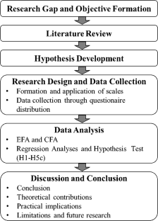
Managing crisis: a qualitative lens on the aftermath of entrepreneurial failure

Does entrepreneurship ecosystem influence business re-entries after failure?
Causal ascriptions and perceived learning from entrepreneurial failure, data availability.
The datasets generated during and/or analyzed during the current study are available from the corresponding author on reasonable request.
Aguzzoli, R., Lengler, J., Sousa, C. M. P., & Benito, G. R. G. (2021). Here we go again: A case study on re-entering a foreign market. British Journal of Management , 32 (2), 416–434. https://doi.org/10.1111/1467-8551.12407
Article Google Scholar
Amankwah-Amoah, J., Boso, N., & Antwi-Agyei, I. (2018). The effects of Business failure experience on successive entrepreneurial engagements: An evolutionary phase model. Group & Organization Management , 43 (4), 648–682. https://doi.org/10.1177/1059601116643447
Amankwah-Amoah, J., Khan, Z., Ifere, S. E., Nyuur, R. B., & Khan, H. (2022). Entrepreneurs’ learning from business failures: An emerging market perspective. British Journal of Management , 33 (4), 1735–1756. https://doi.org/10.1111/1467-8551.12557
Artinger, S., & Powell, T. C. (2016). Entrepreneurial failure: Statistical and psychological explanations [Article]. Strategic Management Journal , 37 (6), 1047–1064. https://doi.org/10.1002/smj.2378
Atuahene-Gima, K., & Murray, J. Y. (2007). Exploratory and exploitative learning in new product development: A social capital perspective on new technology ventures in China. Journal of International Marketing , 15 (2), 1–29. https://doi.org/10.1509/jimk.15.2.1
Baù, M., Sieger, P., Eddleston, K. A., & Chirico, F. (2017). Fail but try again? The effects of age, gender, and multiple–owner experience on failed entrepreneurs’ reentry. Entrepreneurship Theory and Practice , 41 (6), 909–941. https://doi.org/10.1111/etap.12233
Baron, R., & Kenny, D. (1986). The moderator-mediator variable distinction in social psychological research: Conceptual, strategic, and statistical considerations. Journal of Personality and Social Psychology , 51 , 1173–1182. https://doi.org/10.1037//0022-3514.51.6.1173
Baum, J. R., & Locke, E. (2004). The relationship of entrepreneurial traits, skill, and motivation to subsequent venture growth. Journal of Applied Psychology , 89 , 587–598. https://doi.org/10.1037/0021-9010.89.4.587
Article PubMed Google Scholar
Belchior, R. F., & Castro-Silva, H. (2023). The virtuous cycle of entrepreneurial identity and experience - a longitudinal analysis. International Entrepreneurship and Management Journal , 19 (4), 1739–1770. https://doi.org/10.1007/s11365-023-00898-7
Biraglia, A., & Kadile, V. (2017). The role of entrepreneurial passion and Creativity in developing entrepreneurial intentions: Insights from American homebrewers [Article]. Journal of Small Business Management , 55 (1), 170–188. https://doi.org/10.1111/jsbm.12242
Boso, N., Adeleye, I., Donbesuur, F., & Gyensare, M. (2019). Do entrepreneurs always benefit from business failure experience? Journal of Business Research , 98 , 370–379. https://doi.org/10.1016/j.jbusres.2018.01.063
Brüderl, J., Preisendörfer, P., & Ziegler, R. (1992). Survival chances of newly founded business organizations. American Sociological Review , 57 (2), 227–242. https://doi.org/10.2307/2096207
Byrne, O., & Shepherd, D. A. (2015). Different strokes for different folks: Entrepreneurial narratives of emotion, cognition, and making sense of business failure. Entrepreneurship Theory and Practice , 39 (2), 375–405. https://doi.org/10.1111/etap.12046
Cardon, M. S., Gregoire, D. A., Stevens, C. E., & Patel, P. C. (2013). Measuring entrepreneurial passion: Conceptual foundations and scale validation. Journal of Business Venturing , 28 (3), 373–396. https://doi.org/10.1016/j.jbusvent.2012.03.003
Cardon, M. S., & Kirk, C. P. (2015). Entrepreneurial passion as mediator of the self-efficacy to persistence relationship. Entrepreneurship: Theory and Practice , 39 (5), 1027–1050. https://doi.org/10.1111/etap.12089
Cardon, M. S., Stevens, C. E., & Potter, D. R. (2011). Misfortunes or mistakes? Cultural sensemaking of entrepreneurial failure. Journal of Business Venturing , 26 (1), 79–92. https://doi.org/10.1016/j.jbusvent.2009.06.004
Cardon, M. S., Wincent, J., Singh, J., & Drnovsek, M. (2009). The nature and experience of entrepreneurial passion. Academy of Management Review , 34 (3), 511–532. https://doi.org/10.5465/AMR.2009.40633190
Chen, C. C., Greene, P. G., & Crick, A. (1998). Does entrepreneurial self-efficacy distinguish entrepreneurs from managers? [Article]. Journal of Business Venturing , 13 (4), 295–316. https://doi.org/10.1016/S0883-9026(97)00029-3
Cope, J. (2011). Entrepreneurial learning from failure: An interpretative phenomenological analysis. Journal of Business Venturing , 26 (6), 604–623. https://doi.org/10.1016/j.jbusvent.2010.06.002
Corner, P. D., Singh, S., & Pavlovich, K. (2017). Entrepreneurial resilience and venture failure. International Small Business Journal-Researching Entrepreneurship , 35 (6), 687–708. https://doi.org/10.1177/0266242616685604
Costa, P. L., Ferreira, J. J., & de Torres, R. (2023). From entrepreneurial failure to re-entry [Article]. Journal of Business Research , 158 . https://doi.org/10.1016/j.jbusres.2023.113699 . Article 113699.
De Hoe, R., & Janssen, F. (2022). Re-creation after business failure: A conceptual model of the mediating role of psychological capital. Frontiers in Psychology , 13 , 842590. https://doi.org/10.3389/fpsyg.2022.842590
De Sordi, J. O., dos Santos, A. R., de Azevedo, M. C., Jorge, C. F. B., & Hashimoto, M. (2022). Dark, down, and destructive side of entrepreneurship: Unveiling negative aspects of unsuccessful entrepreneurial action. International Journal of Management Education , 20 (3), 100659. https://doi.org/10.1016/j.ijme.2022.100659
Drnovsek, M., Cardon, M. S., & Patel, P. C. (2016). Direct and indirect effects of passion on growing technology ventures. Strategic Entrepreneurship Journal , 10 (2), 194–213. https://doi.org/10.1002/sej.1213
Edeh, F. O., Zayed, N. M., Darwish, S., Nitsenko, V., Hanechko, I., & Islam, K. M. A. (2023). Impression management and employee contextual performance in service organizations (enterprises). Emerging Science Journal , 7 (2), 366–384. https://doi.org/10.28991/esj-2023-07-02-05
Eftekhari, N., & Timmermans, B. (2022). New venture dissolution and the comobility of new venture teams. Small Business Economics , 59 (1), 279–298. https://doi.org/10.1007/s11187-021-00543-z
Eggers, J. P., & Song, L. (2015). Dealing with failure: Serial entrepreneurs and the costs of changing industries between ventures [Article]. Academy of Management Journal , 58 (6), 1785–1803. https://doi.org/10.5465/amj.2014.0050
Espinoza-Benavides, J., & Díaz, D. (2019). The entrepreneurial profile after failure. International Journal of Entrepreneurial Behavior & Research , 25 (8), 1634–1651. https://doi.org/10.1108/ijebr-04-2018-0242
Fanaja, R. A., Pradana, M., Eka Saputri, M., & Utami, D. G. (2023). Knowledge management as driver of women’s entrepreneurial innovativeness. Journal of Human Earth and Future , 4 (1), 1–9. https://doi.org/10.28991/hef-2023-04-01-01
Fan-Osuala, O. (2021). All failures are not equal: Degree of failure and the launch of subsequent crowdfunding campaigns [Article]. Journal of Business Venturing Insights , 16 . https://doi.org/10.1016/j.jbvi.2021.e00260 . Article e00260.
Fisher, R., Merlot, E., & Johnson, L. W. (2018). The obsessive and harmonious nature of entrepreneurial passion. International Journal of Entrepreneurial Behavior & Research , 24 (1), 22–40. https://doi.org/10.1108/IJEBR-01-2017-0011
Franco, M., Haase, H., & António, D. (2021). Influence of failure factors on entrepreneurial resilience in Angolan micro, small and medium-sized enterprises [Article]. International Journal of Organizational Analysis , 29 (1), 240–259. https://doi.org/10.1108/IJOA-07-2019-1829
Fu, H., Xiao, X. H., Ye, B. H. B., Fang, S. J., Li, Y. Q., & Wu, Y. Y. (2023). Stay passionate and carry on: Why passion exhausts and how it can be restored. Current Psychology , 42 (31), 27574–27592. https://doi.org/10.1007/s12144-022-03889-z
Guerrero, M., & Peña-Legazkue, I. (2019). Renascence after post-mortem: The choice of accelerated repeat entrepreneurship [Article]. Small Business Economics , 52 (1), 47–65. https://doi.org/10.1007/s11187-018-0015-7
Haans, R., Pieters, C., & He, Z. L. (2016). Thinking about U: Theorizing and Testing U- and inverted U-shaped relationships in strategy research. Strategic Management Journal , 37 , 1177–1195. https://doi.org/10.1002/smj.2399
Henriquez-Daza, M. C., Capelleras, J. L., & Osorio-Tinoco, F. (2023). Does fear of failure affect entrepreneurial growth aspirations? The moderating role of institutional collectivism in emerging and developed countries [Article]. Journal of Entrepreneurship in Emerging Economies . https://doi.org/10.1108/JEEE-08-2022-0232
He, V. F., Sirén, C., Singh, S., Solomon, G., & von Krogh, G. (2018). Keep calm and carry on: Emotion regulation in entrepreneurs’ learning from failure [Article]. Entrepreneurship: Theory and Practice , 42 (4), 605–630. https://doi.org/10.1111/etap.12273
Hsu, D. K., Shinnar, R. S., & Anderson, S. E. (2019). I wish I had a regular job’: An exploratory study of entrepreneurial regret [Article]. Journal of Business Research , 96 , 217–227. https://doi.org/10.1016/j.jbusres.2018.11.006
Hsu, D. K., Wiklund, J., & Cotton, R. D. (2017). Success, failure, and entrepreneurial reentry: An experimental assessment of the veracity of self-efficacy and prospect theory [Article]. Entrepreneurship: Theory and Practice , 41 (1), 19–47. https://doi.org/10.1111/etap.12166
Hurmerinta, L., Nummela, N., & Paavilainen-Mäntymäki, E. (2024). Boosted by failure? Entrepreneurial internationalisation as a cyclical learning process. European Journal of International Management , 22 (3). https://doi.org/10.1504/ejim.2024.136483
Hwang, K., & Choi, J. (2021). How do failed entrepreneurs cope with their prior failure when they seek subsequent re-entry into serial entrepreneurship? Failed entrepreneurs’ optimism and defensive pessimism and coping humor as a moderator. International Journal of Environmental Research and Public Health , 18 (13), 7021. https://doi.org/10.3390/ijerph18137021
Jenkins, A., & McKelvie, A. (2016). What is entrepreneurial failure? Implications for future research. International Small Business Journal-Researching Entrepreneurship , 34 (2), 176–188. https://doi.org/10.1177/0266242615574011
Jenkins, A. S., Wiklund, J., & Brundin, E. (2014). Individual responses to firm failure: Appraisals, grief, and the influence of prior failure experience. Journal of Business Venturing , 29 (1), 17–33. https://doi.org/10.1016/j.jbusvent.2012.10.006
Karimi, S. (2020). The role of entrepreneurial passion in the formation of students’ entrepreneurial intentions. Applied Economics , 52 (3), 331–344. https://doi.org/10.1080/00036846.2019.1645287
Kawai, N., Sibunruang, H., & Kazumi, T. (2023). Work-family conflict, entrepreneurial regret, and entrepreneurial outcomes during the COVID-19 pandemic [Article]. International Entrepreneurship and Management Journal , 19 (2), 837–861. https://doi.org/10.1007/s11365-023-00846-5
Article PubMed Central Google Scholar
Kiani, A., Ali, A., Biraglia, A., & Wang, D. (2023). Why I persist while others leave? Investigating the path from passion to persistence in entrepreneurship. Journal of Small Business Management , 61 (6), 2818–2848. https://doi.org/10.1080/00472778.2021.1938097
Lafuente, E., Vaillant, Y., Vendrell-Herrero, F., & Gomes, E. (2019). Bouncing back from failure: Entrepreneurial resilience and the internationalisation of subsequent ventures created by serial entrepreneurs. Applied Psychology , 68 (4), 658–694. https://doi.org/10.1111/apps.12175
Lattacher, W., & Wdowiak, M. A. (2020). Entrepreneurial learning from failure. A systematic review. International Journal of Entrepreneurial Behavior & Research , 26 (5), 1093–1131. https://doi.org/10.1108/IJEBR-02-2019-0085
Lee, C. K., Cottle, G. W., Simmons, S. A., & Wiklund, J. (2021). Fear not, want not: Untangling the effects of social cost of failure on high-growth entrepreneurship [Article]. Small Business Economics , 57 (1), 531–553. https://doi.org/10.1007/s11187-020-00324-0
Lin, S., & Wang, S. (2019). How does the age of serial entrepreneurs influence their re-venture speed after a business failure? [Article]. Small Business Economics , 52 (3), 651–666. https://doi.org/10.1007/s11187-017-9977-0
Liu, Y., Li, Y., Hao, X., & Zhang, Y. (2019). Narcissism and learning from entrepreneurial failure [Article]. Journal of Business Venturing , 34 (3), 496–512. https://doi.org/10.1016/j.jbusvent.2019.01.003
Mandl, C., Berger, E. S. C., & Kuckertz, A. (2016). Do you plead guilty? Exploring entrepreneurs’ sensemaking-behavior link after business failure [Article]. Journal of Business Venturing Insights , 5 , 9–13. https://doi.org/10.1016/j.jbvi.2015.12.002
Mantere, S., Aula, P., Schildt, H., & Vaara, E. (2013). Narrative attributions of entrepreneurial failure. Journal of Business Venturing , 28 (4), 459–473. https://doi.org/10.1016/j.jbusvent.2012.12.001
McGrath, R. G. (1999). Falling forward: Real options reasoning and entrepreneurial failure. Academy of Management Review , 24 (1), 13–30. https://doi.org/10.5465/amr.1999.1580438
Mueller, B. A., & Shepherd, D. A. (2016). Making the most of failure experiences: Exploring the relationship between business failure and the identification of business opportunities. Entrepreneurship Theory and Practice , 40 (3), 457–487. https://doi.org/10.1111/etap.12116
Mueller, B. A., Wolfe, M. T., & Syed, I. (2017). Passion and grit: An exploration of the pathways leading to venture success. Journal of Business Venturing , 32 (3), 260–279. https://doi.org/10.1016/j.jbusvent.2017.02.001
Murnieks, C. Y., Mosakowski, E., & Cardon, M. S. (2014). Pathways of passion: Identity centrality, passion, and behavior among entrepreneurs. Journal of Management , 40 (6), 1583–1606. https://doi.org/10.1177/0149206311433855
Newman, A., Obschonka, M., Moeller, J., & Chandan, G. G. (2021). Entrepreneurial passion: A review, synthesis, and agenda for future research. Applied Psychology , 70 (2), 816–860. https://doi.org/10.1111/apps.12236
Pimentel, L., Major, M., & Cruz, A. (2023). Collective action in institutional entrepreneurship: The case of a government agency. Emerging Science Journal , 7 (2), 538–557. https://doi.org/10.28991/esj-2023-07-02-017
Plehn-Dujowich, J. (2010). A theory of serial entrepreneurship. Small Business Economics , 35 (4), 377–398. https://doi.org/10.1007/s11187-008-9171-5
Politis, D. (2005). The process of entrepreneurial learning: A conceptual framework. Entrepreneurship Theory and Practice , 29 (4), 399–424. https://doi.org/10.1111/j.1540-6520.2005.00091.x
Politis, D., & Gabrielsson, J. (2009). Entrepreneurs’ attitudes towards failure - an experiential learning approach. International Journal of Entrepreneurial Behaviour & Research , 15 (4), 364–383. https://doi.org/10.1108/13552550910967921
Rawal, A., Sarpong, D., & Singh, S. K. (2023). Phoenix rising: Rebounding to venture again post firm-failure. Industrial Marketing Management , 112 , 71–84. https://doi.org/10.1016/j.indmarman.2023.05.007
Sarasvathy, S. D., Menon, A. R., & Kuechle, G. (2013). Failing firms and successful entrepreneurs: Serial entrepreneurship as a temporal portfolio [Article]. Small Business Economics , 40 (2), 417–434. https://doi.org/10.1007/s11187-011-9412-x
Saylors, R., Lahiri, A., Warnick, B., & Baid, C. (2023). Looking back to venture forward: Exploring idea and identity work in public failure narratives. Entrepreneurship Theory and Practice , 47 (2), 398–429. https://doi.org/10.1177/10422587211057027 . Article 10422587211057027.
Seckler, C., Funken, R., & Gielnik, M. (2017). Learning from entrepreneurial failure: Integrating emotional, motivational, and cognitive factors. In J. E. Ellingson & R. A. Noe (Eds.), Autonomous learning in the workplace (pp. 54–77). Routledge. https://doi.org/10.4324/9781315674131-4
Shahid, S., & Kundi, Y. M. (2022). Feel dragged out: A recovery perspective in the relationship between emotional exhaustion and entrepreneurial exit [Article]. Journal of Small Business and Enterprise Development , 29 (2), 203–220. https://doi.org/10.1108/JSBED-05-2021-0199
Shepherd, D. A. (2003). Learning from business failure: Propositions of grief recovery for the self-employed. Academy of Management Review , 28 (2), 318–328. https://doi.org/10.5465/amr.2003.9416377
Shepherd, D. A., & Patzelt, H. (2015). Harsh evaluations of entrepreneurs who fail: The role of sexual orientation, use of environmentally friendly technologies, and observers’ perspective taking. Journal of Management Studies , 52 (2), 253–284. https://doi.org/10.1111/joms.12103
Shepherd, D. A., Wiklund, J., & Haynie, J. M. (2009). Moving forward: Balancing the financial and emotional costs of business failure [Article]. Journal of Business Venturing , 24 (2), 134–148. https://doi.org/10.1016/j.jbusvent.2007.10.002
Shirshitskaia, E., Zhou, X., & Zhang, L. (2021). The impact of learning from failure on new ventures’ sustainable development. Frontiers in Psychology , 12 . https://doi.org/10.3389/fpsyg.2021.784518 . Original Research.
Shore, A., Pittaway, L., & Bortolotti, T. (2023). From negative emotions to personal growth: Failure and re-entry into Entrepreneurship. British Journal of Management . https://doi.org/10.1111/1467-8551.12785
Simmons, S. A., Wiklund, J., & Levie, J. (2014). Stigma and business failure: Implications for entrepreneurs’ career choices. Small Business Economics , 42 (3), 485–505. https://doi.org/10.1007/s11187-013-9519-3
Simmons, S. A., Wiklund, J., Levie, J., Bradley, S. W., & Sunny, S. A. (2019). Gender gaps and reentry into entrepreneurial ecosystems after business failure [Article]. Small Business Economics , 53 (2), 517–531. https://doi.org/10.1007/s11187-018-9998-3
Singh, S., Corner, P. D., & Pavlovich, K. (2015). Failed, not finished: A narrative approach to understanding venture failure stigmatization. Journal of Business Venturing , 30 (1), 150–166. https://doi.org/10.1016/j.jbusvent.2014.07.005
Singh, S., Corner, P., & Pavlovich, K. (2007). Coping with entrepreneurial failure. Journal of Management & Organization , 13 (4), 331–344. https://doi.org/10.5172/jmo.2007.13.4.331
Slade Shantz, A., Zietsma, C., Kistruck, G. M., & Cruz, L. B. (2024). Exploring the relative efficacy of ‘within-logic contrasting’ and ‘cross-logic analogizing’ framing tactics for adopting new entrepreneurial practices in contexts of poverty. Journal of Business Venturing , 39 (1). https://doi.org/10.1016/j.jbusvent.2023.106341
Smollan, R., & Singh, S. (2024). How social entrepreneurs respond to enterprise failure [Article]. Journal of Social Entrepreneurship , 15 (1), 1–25. https://doi.org/10.1080/19420676.2021.1890189
Souitaris, V., Zerbinati, S., & Al-Laham, A. (2007). Do entrepreneurship programmes raise entrepreneurial intention of science and engineering students? The effect of learning, inspiration and resources. Journal of Business Venturing , 22 (4), 566–591. https://doi.org/10.1016/j.jbusvent.2006.05.002
Stroe, S., Sirén, C., Shepherd, D., & Wincent, J. (2020). The dualistic regulatory effect of passion on the relationship between fear of failure and negative affect: Insights from facial expression analysis. Journal of Business Venturing , 35 (4), 105948. https://doi.org/10.1016/j.jbusvent.2019.105948
Tu, Y., Hao, X., Rosak-Szyrocka, J., Vasa, L., & Zhao, X. (2023). Obsessive passion, opportunity recognition, and entrepreneurial performance: The dual moderating effect of the fear of failure [Article]. Frontiers in Psychology , 13 , 1037250. https://doi.org/10.3389/fpsyg.2022.1037250
Ucbasaran, D., Shepherd, D. A., Lockett, A., & Lyon, S. J. (2013). Life after business failure: The process and consequences of business failure for entrepreneurs. Journal of Management , 39 (1), 163–202. https://doi.org/10.1177/0149206312457823
Ucbasaran, D., Westhead, P., & Wright, M. (2009). The extent and nature of opportunity identification by experienced entrepreneurs [Article]. Journal of Business Venturing , 24 (2), 99–115. https://doi.org/10.1016/j.jbusvent.2008.01.008
Ucbasaran, D., Westhead, P., Wright, M., & Flores, M. (2010). The nature of entrepreneurial experience, business failure and comparative optimism [Article]. Journal of Business Venturing , 25 (6), 541–555. https://doi.org/10.1016/j.jbusvent.2009.04.001
Vaillant, Y., Mora-Esquivel, R., & Alvarado, M. (2024). The forgetting curve in entrepreneurship: Decaying learning benefits of past entrepreneurial experience. Small Business Economics . https://doi.org/10.1007/s11187-024-00890-7
Walsh, G. S., & Cunningham, J. A. (2017). Regenerative failure and attribution: Examining the underlying processes affecting entrepreneurial learning. International Journal of Entrepreneurial Behavior & Research , 23 (4), 688–707. https://doi.org/10.1108/ijebr-03-2015-0072
Walsh, G. S., & Cunningham, J. A. (2023). Business failure and entrepreneur experiences of passion. International Small Business Journal-Researching Entrepreneurship . https://doi.org/10.1177/02662426231194482
Walter, S. G., & Block, J. H. (2016). Outcomes of entrepreneurship education: An institutional perspective. Journal of Business Venturing , 31 (2), 216–233. https://doi.org/10.1016/j.jbusvent.2015.10.003
Wang, H., Zheng, C., Wu, W., & Sui, F. (2022). How entrepreneurs’ dual narcissism affects new venture growth: The roles of personal initiative and learning from entrepreneurial failure [Article]. Journal of Organizational Change Management , 35 (7), 1125–1146. https://doi.org/10.1108/JOCM-10-2021-0313
Williams, T. A., Thorgren, S., & Lindh, I. (2020). Rising from failure, staying down, or more of the same? An inductive study of entrepreneurial reentry. Academy of Management Discoveries , 6 (4), 631–662. https://doi.org/10.5465/amd.2018.0047
Yamakawa, Y., & Cardon, M. S. (2015). Causal ascriptions and perceived learning from entrepreneurial failure. Small Business Economics , 44 (4), 797–820. https://doi.org/10.1007/s11187-014-9623-z
Yamakawa, Y., Peng, M. W., & Deeds, D. L. (2015). Rising from the ashes: Cognitive determinants of venture growth after entrepreneurial failure [Article]. Entrepreneurship: Theory and Practice , 39 (2), 209–236. https://doi.org/10.1111/etap.12047
Yang, T., & Aldrich, H. E. (2012). Out of sight but not out of mind: Why failure to account for left truncation biases research on failure rates [Article]. Journal of Business Venturing , 27 (4), 477–492. https://doi.org/10.1016/j.jbusvent.2012.01.001
Yao, K., Li, X., & Liang, B. (2021). Failure learning and entrepreneurial resilience: The moderating role of firms’ knowledge breadth and knowledge depth [Article]. Journal of Knowledge Management , 25 (9), 2141–2160. https://doi.org/10.1108/JKM-10-2020-0772
Zhao, H., & Wibowo, A. (2021). Entrepreneurship resilience: Can psychological traits of entrepreneurial intention support overcoming entrepreneurial failure? Frontiers in Psychology , 12 , Article 707803. https://doi.org/10.3389/fpsyg.2021.707803
Download references
Acknowledgements
The first author would like to acknowledge the financial support of the National Natural Science Foundation of China (Grant No: 72172165) and the Natural Science Foundation of Guangdong Province, China (Grant No: 2024A1515011283).
Author information
Authors and affiliations.
School of Business, Sun Yat-sen University, No.135 Xingang West Road, Guangzhou, 510275, Guangdong, China
Hui Fu, Min Xu, Shaoshuai Zhang, Hui Yang & Yuan Wei
You can also search for this author in PubMed Google Scholar
Corresponding author
Correspondence to Yuan Wei .
Ethics declarations
Ethical approval.
All procedures performed in studies involving human participants were in accordance with the ethical standards of the institutional and/or national research committee and with the 1964 Helsinki Declaration and its later amendments or comparable ethical standards.
Informed consent
We’ve obtained inform consent from all individual participants included in the study.
Conflict of interest
There is no conflict of interest.
Additional information
Publisher’s note.
Springer Nature remains neutral with regard to jurisdictional claims in published maps and institutional affiliations.
Rights and permissions
Springer Nature or its licensor (e.g. a society or other partner) holds exclusive rights to this article under a publishing agreement with the author(s) or other rightsholder(s); author self-archiving of the accepted manuscript version of this article is solely governed by the terms of such publishing agreement and applicable law.
Reprints and permissions
About this article
Fu, H., Xu, M., Zhang, S. et al. Unraveling entrepreneurial comebacks: the curvilinear relationship between entrepreneurial failure and reentry intention. Curr Psychol (2024). https://doi.org/10.1007/s12144-024-06511-6
Download citation
Accepted : 31 July 2024
Published : 27 August 2024
DOI : https://doi.org/10.1007/s12144-024-06511-6
Share this article
Anyone you share the following link with will be able to read this content:
Sorry, a shareable link is not currently available for this article.
Provided by the Springer Nature SharedIt content-sharing initiative
- Entrepreneurial failure
- Reentry intention
- Learning from failure
- Entrepreneurial passion
- Find a journal
- Publish with us
- Track your research

An official website of the United States government
The .gov means it’s official. Federal government websites often end in .gov or .mil. Before sharing sensitive information, make sure you’re on a federal government site.
The site is secure. The https:// ensures that you are connecting to the official website and that any information you provide is encrypted and transmitted securely.
- Publications
- Account settings
Preview improvements coming to the PMC website in October 2024. Learn More or Try it out now .
- Advanced Search
- Journal List
- ACS AuthorChoice
- PMC11342373
Development and Application of a Liquid Chromatography–Tandem Mass Spectrometry Method for the Analysis of 20 Perfluoroalkyl Substances in Fruit and Vegetables at Sub-Parts-per-Trillion Levels
Associated data.

In response to the European Food Safety Authority’s establishment of a tolerable weekly intake (TWI) for the sum of PFOA, PFNA, PFHxS, and PFOS, a method was developed to quantify and confirm 20 PFASs at the sub-parts-per-trillion level in fruit and vegetables. Improved sensitivity was achieved by (i) increasing the sample intake, (ii) decreasing the solvent volume in the final extract, and (iii) using a highly sensitive mass spectrometer. Except for PFTrDA, target PFASs could be quantitatively determined with an apparent recovery of 90–119%, limits of quantitation down to 0.5 ng/kg, and a relative standard deviation under within-laboratory reproducibility conditions of <28%. The method was successfully applied to 215 fruit and vegetable samples obtained from local grocery stores and markets. Leafy vegetables prove to be the main vegetable category responsible to PFAS exposure, mainly of PFOA, followed by PFHpA and PFHxA.
Introduction
Per- and polyfluoroalkyl substances (PFASs) are an extensive class of synthetic chemicals known for their chemical and heat resistance as well as their ability to strongly reduce surface tension. They have been extensively manufactured and utilized in various industries due to these desirable properties. 1 They have been used in the production of non-stick cookware, waterproof clothing, and fire-fighting foams, among other products.
Due to increasing global concern about the potential negative health effects of PFASs, the European Food Safety Authority (EFSA) conducted a new risk assessment of PFASs in food. EFSA derived a tolerable weekly intake (TWI) of 4.4 ng/kg of body weight per week for the sum of four PFASs. These PFASs are perfluorooctanoic acid (PFOA), perfluorononanoic acid (PFNA), perfluorohexanesulfonic acid (PFHxS), and perfluorooctanesulfonic acid (PFOS); the so-called “EFSA-4”. It was shown that current exposure of a large part of the European Union (EU) population exceeds this TWI, even when applying the lower-bound principle (i.e., assuming that non-detected levels are equal to zero). The upper-bound exposure [i.e., assuming that non-detected levels equal the concentration of the limit of quantification (LOQ)] was much higher, implying a large uncertainty in the assessment and the need to apply more sensitive analytical methods.
The stringent requirements of the low TWI necessitate the use of highly sensitive analytical methods with low limits of quantification. When methods with relatively high LOQs are used, the majority of analyses yield non-detectable results. Typically, exposure assessments are conducted under an upper-bound scenario, where samples with non-detects are assumed to contain PFASs at the LOQ. Following this principle, if the method’s LOQs are too high, PFAS exposure can surpass the new TWI by many orders of magnitude, even in the absence of detected PFASs in the samples.
Considering the potential harm associated with PFASs, even at low concentrations, there is an urgency to develop analytical methods with low detection limits for various food products, as emphasized by EFSA. 2 The European Union Reference Laboratory for Persistent Organic Pollutants in Feed and Food (EURL-POPs) has issued guidance on PFAS analysis, specifying that for fruit and vegetables, LOQs should be ≤5 ng/kg for PFNA, ≤10 ng/kg for PFOA and PFOS, and ≤15 ng/kg for PFHxS. 3 Furthermore, laboratories are encouraged to aim for even lower LOQs, specifically ≤1 ng/kg for PFOA and PFNA, ≤2 ng/kg for PFOS, and ≤4 ng/kg for PFHxS. These latter LOQs have been adopted by Commission Regulation EU 2022/1431 as mandatory for monitoring purposes. 4
Within the food domain, according to EFSA, 2 fish and other seafood are the main sources of exposure to PFOA and PFOS, followed by eggs, meat products, and fruit. Notably, fruit and vegetables are an important source of exposure to PFOA, because of their substantial consumption compared to other foods.
Recent literature reviews have explored analytical methodologies for PFAS analysis and their occurrence in various sources, including food 5 , 6 Furthermore, in recent years, there has been an expanded focus on examining the presence and transfer of PFASs in fruit and vegetables. Various studies describe methodologies to monitor PFAS levels in fruit and vegetables. 7 − 20 Additionally, some studies have documented analytical methods to study the transfer of several PFASs from contaminated irrigation water to crops. 21 − 23 Regrettably, most of the developed methods did not meet the targeted and/or proposed LOQs currently required by the EURL-POPs 3 and commission regulation EU 2022/1431. 4 Most methods were validated at relatively high concentration levels, and/or no fit-for-purpose validation was reported. Table 1 offers a comparison of recent studies on the analysis of PFASs in fruit, vegetables, and other plant material, highlighting the substantial variability in analytical characteristics of current methods. As a result, only scarce high-quality quantitative data on PFASs in vegetables at required concentration levels was available prior to the study presented here.
| detection/quantification limit | ||||||||
|---|---|---|---|---|---|---|---|---|
| authors | matrix | extraction method | clean-up procedure | instrumentation | targeted PFAS | value | methodology | lowest recovered spike level |
| Zhou et al. | vegetables | acetonitrile + formic acid | Sin-QuEChERS (PSA, C18, and GCB) | UHPLC–MS/MS | 20 PFASs, including PFCAs, and PFSAs | 0.003–0.034 μg/kg (LOQ) | 10× S/N | 0.1 μg/kg |
| Li et al. | vegetables | methanol | online SPE | UHPLC–MS/MS | 21 PFASs, including PFCAs, PFSAs, and FTSs | 0.002–0.008 μg/kg (LOD) | 3× SD of spike (0.2 μg/kg) | 0.2 μg/kg |
| Nassazzi et al. | plant material | methanol | ENVI carb cartridge | UHPLC–MS/MS | 24 PFASs, including PFCAs, PFSAs, FASAs, and FTSs | 0.01–11.0 μg/kg (LOQ) | 10× S/N | 0.025 μg/kg |
| Meng et al. | fruit and vegetables | methanol + ammonium hydroxide | WAX SPE | UHPLC–MS/MS | 45 PFASs, including PFCAs, PFSAs, PFEAs, FASAs, FTSs, FTCAs, and PFESAs | 0.025 to 0.25 ng/g (LOQ) | lowest recovered solvent standard × matrix effect | 1 μg/kg |
| Piva et al. | vegetables | acetonitrile + formic acid | WAX SPE | UHPLC–MS/MS | 22 PFASs, including 3 FTSs | 0.05–0.5 μg/kg (LOQ) | 10× S/N | 1 μg/kg |
| Zacs et al. | fruit and vegetables | acetonitrile + NaOH | WAX SPE | nano-LC–nano-ESI–Orbitrap MS | EFSA-4 | 0.001–0.002 μg/kg | lowest validated spike | 0.001 μg/kg |
In the current study, a method was developed and validated to detect and quantify 20 PFASs, including PFOA, PFNA, PFHxS, and PFOS, at the low ppt (ng/kg) level in a wide range of fruit and vegetables (see SI-2 of the Supporting Information). This study is the first description of a method that can achieve the very low detection limits required for human exposure assessments of PFAS via fruit and vegetables. The achievement of such low detection limits is especially challenging as background contamination of commonly applied PFAS becomes apparent. Also, we demonstrate an extensive validation protocol to include a wide range of vegetables. The method was subsequently applied to a selection of fruit and vegetables obtained from local grocery stores and weekly markets ( n = 215).
Materials and Methods
Methanol (MeOH) and acetonitrile of UHPLC/MS grade were purchased from Actu-All Chemicals (Oss, Netherlands). UHPLC/MS grade water was procured from Biosolve (Valkenswaard, Netherlands). All other chemicals were obtained from Merck (Darmstadt, Germany). A 2% ammonium hydroxide solution was prepared by diluting a 25% ammonium solution 12.5 times in acetonitrile. A 25 mM sodium acetate buffer was prepared by dissolving 3.40 g of sodium acetate trihydrate in 1 L of water and adjusting to pH 4 with glacial acetic acid. A 4 M hydrochloric acid solution was prepared by diluting 3.3 mL of 37% HCl to 10 mL with water, and lower concentrations were prepared by diluting this solution. Mobile phase A was a 20 mM ammonium acetate in water solution, was prepared by dissolving 1.54 g of ammonium acetate in 1 L of water. Mobile phase B was methanol.
Reference Standards
All reference standards were obtained from Wellington Laboratories (Guelph, Ontario, Canada). The following perfluoroalkyl carboxylic acids (PFCAs) were used in this study: perfluoropentanoic acid (PFPeA, C 5 ), perfluorohexanoic acid (PFHxA, C 6 ), perfluoroheptanoic acid (PFHpA, C 7 ), PFOA (C 8 ), PFNA (C 9 ), perfluorodecanoic acid (PFDA, C 10 ), perfluoroundecanoic acid (PFUnDA, C 11 ), perfluorododecanoic acid (PFDoDA, C 12 ), perfluorotridecanoic acid (PFTrDA, C 13 ), and perfluorotetradecanoic acid (PFTeDA, C 14 ). All PFCAs were obtained as a mixture of 2 μg/mL in MeOH.
The following perfluoroalkyl sulfonic acids (PFSAs) were used in this study: perfluorobutanesulfonic acid (PFBS, C 4 ), PFHxS (C 6 ), perfluoroheptanesulfonic acid (PFHpS, C 7 ), PFOS (C 8 ), and perfluorodecanesulfonic acid (PFDS, C 10 ). These PFSAs were obtained as individual solutions of their sodium salts (except PFBS, which is a potassium salt) of 2 μg/mL in MeOH. Additionally, a few other PFASs were included in this study. Those being: perfluorooctanesulfonamide (PFOSA), hexafluoropropylene oxide–dimer acid (HFPO–DA), also known as GenX technology, Sodium dodecafluoro-3 H -4,8-dioxanonanoate (NaDONA), sodium dodecafluoro-3 H -4,8-dioxanonanoate (9Cl-PF3ONS), and sodium dodecafluoro-3 H -4,8-dioxanonanoate (11Cl-PF3OUdS). These compounds were also obtained at a concentration of 2 μg/mL in MeOH. All reference compounds have a chemical purity of at least 98%.
Isotopically labeled compounds were used as internal standards in this study. A mixture containing the following compounds was obtained at a concentration of 2 μg/mL in methanol: 13 C 2 -PFHxA, 13 C 4 -PFOA, 13 C 5 -PFNA, 13 C 2 -PFDA, 13 C 2 -PFUnDA, 13 C 2 -PFDoDA, 18 O 2 -PFHxS, and 13 C 4 -PFOS. Additionally, 13 C 3 -PFPeA, 13 C 4 -PFHpA, 13 C 3 -PFBS, and 13 C 3 -HFPO–DA were obtained as individual solutions at the same concentration. Isotopically labeled 13 C 8 -PFOA and 13 C 8 -PFOS standards were used as injection checks (2 μg/mL). All labeled compounds had a chemical purity of at least 98% and isotopic purities of at least 99% for 13 C and 94% for 18 O.
Sample Preparation
Ten grams of sample were transferred to a 50 mL polypropylene (PP) centrifuge tube (Greiner Bio-One, Kremsmünster, Austria). The sample was then fortified with 50 μL of internal standard solution (1 ng/mL) and 0.5 mL of 200 mM sodium hydroxide solution was added, followed by 10 mL of MeOH. The mixture was vortexed for 1 min in a multivortex mixer (VWR, VX-2500 Vulti-Tube Vortexer, Radnor, PA, U.S.A.), followed by 15 min of ultrasonication at room temperature (in an ultrasonic bath by Branson, Danbury, CT, U.S.A.) and 30 min of shaking on a rotary tumbler (REAX-2, Heidolph, Schwabach, Germany). After the extraction, 100 μL of formic acid was added and the mixture was centrifuged for 10 min at 3600 rpm at 10 °C (Rotixa 500 RS, Hettich Zentrifugen, Westphalia, Germany). The supernatant was then carefully decanted into a 50 mL PP tube that contained 25 mL of HPLC-grade water. The extract was mixed and centrifuged again if cloudy, before the cleanup.
For cleanup and further concentration of the sample, a Strata-X-AW cartridge (mixed mode weak anion exchange, 200 mg per 6 mL, 33 μm; Phenomenex, Torrance, CA, U.S.A.) was conditioned with 8 mL MeOH and then 8 mL of 0.04 M HCl. The extract was transferred onto the cartridge and slowly passed through (if necessary, by applying a vacuum) to allow interaction between the SPE material and the PFASs. The cartridge was then rinsed with 5 mL of 25 mM sodium acetate buffer, followed by 3 mL of 0.04 M HCl in MeOH. The PFASs were eluted from the cartridge using 5 mL of 2% ammonium hydroxide in acetonitrile and collected into a 14 mL PP tube (Greiner Bio-One, Kremsmünster, Austria).
The solvent was evaporated (at 40 °C using nitrogen gas) using a TurboVap LV Evaporator (Zymark, Hopkinton, MA, U.S.A.). After evaporation to dryness, 80 μL MeOH, 270 μL ammonium acetate buffer (20 mM), and 50 μL of the injection standard mixture (1 ng/mL) (containing 13 C 8 -PFOA and 13 C 8 -PFOS) were added. The residues were then reconstituted by rigorous mixing (vortex mixer) and 5 min of ultrasonication. The final extract was passed through a 0.45 μm regenerated cellulose syringe filter (Whatman, Little Chalfont, Buckinghamshire, U.K.) before LC–MS/MS analysis.
UPLC–MS/MS
The UPLC–MS/MS analysis was performed using a Sciex ExionLC UPLC system (Sciex, Framingham, MA, U.S.A.). A Luna Omega PS C18 analytical column (100 Å, 100 × 2.1 mm inner diameter, 1.6 μm, Phenomenex, Torrance, CA, U.S.A.) was used to separate the PFASs at a column temperature of 40 °C. Additionally, a Gemini C18 analytical column (110 Å, 50 × 3 mm inner diameter, 3 μm, Phenomenex) was used as an isolator column, placed between the pump and the injector valve to isolate and delay potential PFAS contamination eluting from the LC system parts prior to the injection valve. The gradient: 0–1.5 min, 20% mobile phase B, 1.5–9.5 min, linear increase to 98% B with a final hold of 1.4 min. The gradient was returned to its initial conditions within 0.1 min and the column was allowed to equilibrate for 2.5 min before the next injection was initiated, resulting in a total run of 13.5 min. The flow rate was 0.5 mL/min and the injection volume 20 μL.
The detection of PFASs was done using MS/MS on a Sciex QTRAP 7500 system in negative electrospray ionization (ESI−) mode. The ion spray voltage, curtain gas, source temperature, gas 1, gas 2, and collision gas were set at −1500 V, 45 psi, 400 °C, 40, 80, and 9 psi, respectively. To fragment the PFASs, collision-induced dissociation (CID) was used with argon as the collision gas. The analysis was performed in multiple reaction monitoring (MRM) mode, using two mass transitions per component (except for PFPeA), which were selected based on the abundance of the signal and the selectivity of the transition. Additional information on the MRM transitions, entrance potential, collision energy, and cell exit potential can be found in Table S1 of the Supporting Information. The data were acquired using SciexOS and processed using MultiQuant software (SCIEX, Framingham, MA, U.S.A.).
Blank Level Management
To reduce the risk of contamination through material selection, all fluoropolymer containers (tubes, vials, etc.) and devices (filters, pipets, etc.) were excluded from the method, if possible. The analysts did not wear any cosmetics or PFAS-containing clothing during sample handling, as required by EU regulations (EU) 2022/1428. Although no significant concentrations of PFASs were observed in the procedural blanks, except for PFBA, PFPeA, and small amounts of PFOA, it is recommended to test solvents and chemicals for PFASs prior to method development. Several sources with low-contamination were identified and eliminated. This test became essential only after the need for very low detection limits.
To test and correct for incidental contamination originating from the laboratory or laboratory consumables, blank chemical preparations (procedural blanks) were carried out in duplicate each day. The signal of all samples was corrected with the average response of the procedural blanks. The impact of interfering signals becomes more pronounced with extremely low method detection limits.
This validation study aimed to cover a broad range of commonly consumed fruit and vegetables in the Netherlands. As a basis for the validation of the EURL POPs guidance document on PFAS analysis in food 3 was applied. The validation was done more extensively than required by that document.
The following parameters related to a quantitative confirmatory method were determined: selectivity, stability, robustness, apparent recovery (trueness based on spiked samples), within-laboratory reproducibility (expressed as relative standard deviation, RSD RL ), repeatability (expressed as relative standard deviation, RSD r ), limit of detection (LOD), limit of quantification (LOQ), and limit of confirmation (LOC).
Validation Design
The method was characterized as a quantitative confirmatory method and the validation was designed to challenge fit-for-purpose for this goal. Fruit and vegetables were selected and subdivided into five matrix categories: leafy vegetables, fruit, root vegetables, bulb vegetables, and leek, and “other vegetables” mostly containing fruiting vegetables, legumes, and cabbage. The validation of each matrix category was performed on a single day, yielding a total of 5 validation days ( Table 2 ). For each category, a representative matrix was selected for preparation of the matrix-fortified calibration (P1, Table 2 ). Furthermore, an additional six matrices (P2–P7, Table 2 ) of each category were analyzed as is (blank) and with the addition of all 20 PFASs at 2.5, 50, and 500 ng/kg. A detailed overview of the validation design is given in Table S2 of the Supporting Information.
| number | leafy vegetables | bulb vegetables and leek | root vegetables | fruit | other vegetables |
|---|---|---|---|---|---|
| P1 (MFS) | spinach | onion | potato | apple | zucchini |
| P2 | endive | onion | beets (peeled) | strawberry | cauliflower |
| P3 | kale | leek | beets (unpeeled) | white grape | broccoli |
| P4 | iceberg lettuce | garlic | carrot (peeled) | plum | snow peas |
| P5 | Turkish lettuce | red onion | carrot (unpeeled) | pear | rhubarb |
| P6 | chard | scallions | potato (peeled) | red berries | pumpkin |
| P7 | Batavia lettuce | chives | potato (unpeeled) | apple | cucumber |
Quantification
One specific sample batch (P1, Table 2 ) was selected for matrix-fortified standard calibration on each day. The matrix fortified standards (MFS calibration standards) included the following concentration levels to cover a wide concentration range: 0, 0.5, 1.0, 2.5, 5.0, 10, 25, 50, 100, 500, 1000, and 2000 ng/kg. Based on the PFAS concentration in the samples, the lower or higher end of the calibration line was used for quantification. Quantitative results were achieved using the matrix-fortified standard calibration approach, which involved correcting the signals (peak area) of the individual PFASs with the corresponding isotopically labeled internal standards. This correction accounts for differences in the recovery, ionization, and other matrix influences. For PFTrDA, PFHpS, PFDS, DONA, 9Cl-PF3ONS, and 11Cl-PF3OUdS no labeled internal standard were available. For these compounds, an internal standard was selected based on their retention time and chemical similarities. Retention time was the most important factor. The internal standards used per analyte are included in Table S1 of the Supporting Information.
Confirmation of Peak Identity
For confirmatory analysis, criteria have been established in the EURL-POPs guidance document 3 for the maximum allowed deviation of the relative abundance of both diagnostic ions (ion ratio) resulting from an unknown sample. The maximum allowed deviation is 30%. Furthermore, the relative retention time of a PFAS should not deviate more than 1% from the reference relative retention time. To assess the possibility of confirming the identity of a detected compound using the presented method the average ion ratio and the average relative retention time of the matrix-fortified standard calibration samples was used as the reference value.
Selectivity, Stability, and Robustness
The EURL-POPs guidance document 3 states that analytical methods should demonstrate the ability to reliably and consistently separate the analytes of interest from other coextracted and possibly interfering compounds that may be present. It is known that PFOS detection may suffer from a coeluting interference of taurodeoxycholic acid (TDCA), which is a bile acid with the same transition as the most sensitive PFOS transition ( m / z 499 > 80). 28 This bile acid is particularly prominent in eggs. 29 In this method TDCA was chromatographically separated from PFOS and the mass transition m / z 499 > 99 was applied for quantitative purposes, preventing any interference. Moreover, it is unlikely that this bile acid interference occurs in fruit and vegetables. Additionally, it is noteworthy that although the m / z 499 to 99 transition is 75% less sensitive, it offers much greater specificity, resulting in fewer observed interferences in general. The robustness of the method was challenged by including many different fruit and vegetables. Furthermore, the validation was carried out on five different days and by three different technicians.
The stability of the PFASs in the samples and solvent solutions was not tested as it is generally agreed upon that these substances are very persistent. From the PFASs included in this study, only HFPO–DA is known to degrade to heptafluoropropyl 1,2,2,2-tetrafluoroethyl ether in aprotic polar solvents, such as dimethyl sulfoxide, acetone, and to a lesser extent in acetonitrile; with 100% degradation after approximately 15 h. 30 , 31
Additionally, Zhang et al. showed that the degradation of HFPO–DA in acetonitrile was negligible in the presence of water (>20%), suggesting that acetonitrile can be used as a solvent for sample preparation when the water content is >20%. 31 In our experiments, the lowest water concentration in acetonitrile of the extract is approximately 8%, under alkaline conditions. Under these conditions, we therefore assume that the degradation of HFPO–DA is limited, but not excluded. To test this hypothesis, a single-factor ANOVA was performed on the relative standard deviation of the signal of the internal standards for HFPO-DA, PFOA, and PFOS; two PFASs that are considered to be very persistent. We assume that there would be a larger variance in signal intensity of HFPO-DA, when degradation is a critical factor.
Apparent Recovery (Trueness), Repeatability, and Within-Laboratory Reproducibility
For the calculation of apparent recovery (trueness), repeatability, and within-laboratory reproducibility for each PFAS the quantitative data obtained from the samples spiked at 2.5, 50, and 500 ng/kg of each analyte was used. The apparent recovery for each sample was calculated by dividing the calculated concentration by the actual spiked concentration, in some cases after correction for a signal found in the procedural blank or the non-fortified sample. The reported apparent recovery for a specific PFAS is the average of all spiked samples at a concentration level. The relative standard deviation under repeatability conditions (RSD r ) was calculated from all the individual analyzed matrices within a single matrix category for each concentration level. The relative standard deviation under within-laboratory reproducibility conditions (RSD RL ) was calculated from all matrices at each concentration level. Note that in this validation design, for repeatability calculations different matrices are included. Therefore, the result is an overestimation of the actual repeatability. This approach was used to determine the overall performance of the method with a very high variation in types of fruit and vegetables.
The performance criteria were established in advance and derived from the EURL POPs guidance document. 3 The guidance document differentiates analysis for compliance testing and analysis for monitoring purposes. Compliance testing relates to the EFSA-4 PFASs at the regulatory level. As for fruit and vegetables, no regulatory limits have been established, in this validation the method performance criteria for monitoring apply. The apparent recovery must lie between 65 and 135%, RSD RL should be ≤25%. No criterion for RDS r is established.
Limit of Detection, Quantification, and Confirmation
As this method would be applied to food exposure studies, it is crucial to establish limits for determining the absence and presence of specific substances. To accomplish this, we have adopted the approach previously described by Berendsen et al., 32 with a focus on the LOQ and LOC.
The LOQ represents the concentration at which a quantitative result can be obtained, typically based on a single ion transition, whereas confirmation of the identity at this concentration may not be possible. Concentrations at or below the LOQ are used to report the absence of a substance, based on this single ion transition. The LOC is considered to be the lowest concentration level of a PFAS at which it complies with the confirmatory criteria, as described under “ Confirmation of Peak Identity ”. 33
For some substances, signals in the procedural blanks, originating from e.g. solvents, are common. Therefore, we applied two different strategies to determine the LOQ and LOC. One approach is employed when no substantial signal is observed in the procedural blanks, while the other is used when a substantial signal is detected in the procedural blanks.
If no signal of a specific PFAS is detected in the procedural blank samples, we established the LOQ as the lowest spiked concentration in the MFS calibration line with a signal-to-noise ratio ≥6. 34 The LOC, in this case, is defined as the lowest spiked concentration in the MFS calibration line, meeting the confirmatory requirements.
On the other hand, when a signal is detected in the procedural blank, we follow the guidelines set by the EURL, 3 which provides that the contribution of blank levels should not exceed 30% of the levels in the samples analyzed in the accompanying batch. In such a case, the LOQ was determined by multiplying the concentration of the PFAS in the procedural blank by a factor of 3.3. The LOC remains as the lowest spiked concentration in the MFS calibration line that meets the confirmatory requirements. If, in this scenario, the determined LOC is lower than the LOQ, it is set equal to the LOQ. In any case, the determined LOQ and LOC are assessed by comparing them to the results of the spiked validation samples and adjusted accordingly if needed (e.g., in case the LOQ derived from the MFS seems unachievable or unrealistic as that is only derived from a single matrix).
Application
The developed method was applied to the analysis of 215 fruit and vegetables obtained from Dutch grocery stores and weekly markets, of which 35 leafy vegetables, 25 root vegetables, 23 bulb vegetables and leek, 50 fruit, and 82 other vegetables. The samples were collected and analyzed in 2021. A list of samples and their land of origin is included in SI-4 of the Supporting Information.
Results and Discussion
Method development.
Not all substances recommended by the EURL-POPs were included in this study, such as some long-chain PFSAs (perfluoroalkyl sulfonic acids) and next-generation PFASs. 3 These compounds were at the time unavailable to the laboratory.
Achieving the required LOQs for fruit and vegetables poses a significant challenge due to their exceptionally low target thresholds and diverse matrices. Our strategy to achieve the lowest possible LOQs involves increasing the concentration factor of samples by increasing the sample intake and lowering the extract reconstitution volume. However, practical constraints, such as the capacities of extraction tubes, shaking equipment, and centrifuges, limit the sample intake volume.
It is crucial to fine-tune the extraction process as well, focusing on optimizing the solvent and solvent-to-sample ratio to allow the extract to run through the solid-phase extraction (SPE) cartridge. In the case of certain fruit and vegetables, the final extracts exhibited turbidity. A filtering step was therefore a requirement. Even after filtering, some extracts were somewhat turbid, demonstrating that the practical limitations of the method had been reached. Final extracts that were still turbid were shortly centrifuged, using a high-speed centrifuge, at 12 000 rpm.
The extraction process presented particular challenges when dealing with leafy greens, as they tended to yield cloudy extracts. Moreover, the preparation of certain leafy greens, like chives and leek, occasionally proved cumbersome, especially during the grinding process, due to their unique textures and structures. The fibrous nature and large, flat surface areas of some leaves made grinding a labor-intensive task. These combined factors contribute to the complexity of the analytical process in this study.
To gain insights into the performance of the analytical process, we introduced internal standards into the samples prior to the preparation stage and added injection standards just before the sample injection. The injection standard consists of two isotopically labeled analogs of PFOS and PFOA (see SI-1 of the Supporting Information). Assessing the relative abundance of the internal- and injection standards, we found absolute recoveries ranging between 41 and 79% for PFOA and 32 and 63% for PFOS. Notably, bulb vegetables exhibited substantially lower absolute recoveries (32–53%) compared to other fruit and vegetables. Matrix effects for PFOA and PFOS were determined by comparing the injection standard added to sample matrices after cleanup with the injection standard added to the procedural blank, revealing a range from 32% for bulb vegetables to 157% for leafy vegetables. The matrix effect could only be determined for PFOA and PFOS since isotopically labeled variants ( 13 C 8 ) of those PFAS were included in the injection standard.
The hydrophobic nature of the PFASs included in this study is very diverse, as indicated by the octanol–water partitioning coefficient ( K ow ) ranging from 3.4 for PFPeA to 7.15 for PFUnDA, 35 with higher values for the longer chain PFASs (no data available). 36 Prior work by Zenobio et al. highlighted the adsorption of hydrophobic PFASs to container surfaces. 36 From the recovery experiments in the current study, this effect was observed for the long-chain PFASs (≥C 12 ). Approximate 50% MeOH is required to keep these PFASs in solution in the glass LC vial. However, a high organic solvent percentage in the final extract jeopardizes the chromatographic separation of short-chain PFAS. To address this, we opted for a final extract composition containing 32.5% MeOH, ensuring satisfactory peak shapes for the early eluting PFASs and an acceptable recovery for the long-chain PFASs.
Given that long-chain PFASs (≥C 12 ) were anticipated to be present in crops to a lesser extent than shorter chain PFASs, 37 an absolute recovery within the range of approximately 5 to 20% compared to PFOA was deemed an acceptable threshold. PFHxDA (perfluorohexadecanoic acid) and PFODA (perfluorooctadecanoic acid) were originally included in the method development. However, it demonstrated extremely low absolute recovery under the current conditions. Given the unlikely accumulation of these compounds in fruit or vegetables, we adjusted the method’s focus toward more hydrophilic PFASs. During method development and validation, perfluorobutyric acid (PFBA) was also considered. Unfortunately, it displayed severe background signals in all injections, restricting the method’s applicability (see SI-3 of the Supporting Information). Consequently, PFBA was excluded from the method. A MRM chromatogram of a potato sample spiked at 10 ng/kg with all 20 PFASs is presented in Figure Figure1 1 . In SI-3 of the Supporting Information, example chromatograms are included of unspiked samples, and at 1 ng/kg.

MRM chromatogram of all 20 PFASs in a spiked potato sample at 10 ng/kg. PFOSA is not visible in the current view but elutes after 10 minutes.
In examining the selectivity challenges posed by both PFBA and PFPeA, which have only a single sufficiently abundant product ion in MS/MS detection, the method’s limitation becomes apparent. It becomes difficult to conclusively determine whether an observed signal is related to the presence of an interfering substance or if PFBA or PFPeA is genuinely present in the chromatogram. The few publications that integrated PFBA and PFPeA in their methods and reported their presence in fruit and vegetables share this limitation, often without addressing the lack of selectivity. Therefore, findings related to PFBA and PFPeA should be interpreted with caution. To address this selectivity issue, we introduced the ion transition from precursor ion mass to precursor ion mass at low collision energy for PFPeA, allowing for the calculation of relative ion abundance. It is important to note that this approach deviates from EURL guidance requirements, and for definitive confirmation, an additional orthogonal separation or alternative detection technique must be employed.
In the current study, the inclusion of PFOSA, a neutral PFAS, needs some extra clarification. As a neutral compound, PFOSA does not interact with the anion exchange mechanism of the SPE cleanup procedure, only interacting with the backbone material based on its hydrophobicity. During the SPE procedure, the cartridge is flushed with methanol, causing a large fraction of PFOSA to elute from the column. Only a small part is eluted in the final elution step. This fraction is sufficient for the quantitative determination of PFOSA, but due to the lower absolute recovery, only with a higher detection limit and a larger variance in recovery. The PFOSA recovery can be improved by collecting, evaporating, reconstituting, and injecting the methanolic wash fraction separately.
Additionally, another challenging compound to analyze is HFPO-DA, known for its susceptibility to degradation under specific conditions. To test for the degradation of HFPO-DA, a single-factor ANOVA was conducted on the relative standard deviation of the signals of the internal standards for HFPO-DA, PFOA and PFOS. No significant variance was observed in the signal of the internal standard of HFPO-DA compared to PFOA and PFOS ( p = 0.39, among all matrix categories). Consequently, the null hypothesis was rejected, suggesting that any potential degradation of HFPO-DA is negligible during the evaporation of the extracts. This ANOVA analysis was based on a total of 10 individual measurements, with all matrix categories included twice.
The determined LOQs for each matrix category are presented in Table 3 . We selected the definition of the LOQ fitting the aim of this research: exposure assessment. A clear definition of the LOQ is crucial to obtain reliable data as requested by the risk assessors. Unfortunately, the definition of the LOQ and the determination of it is not harmonized. This commonly results in underestimations of the actual LOQ, since often system-LOQs are used, instead of method-LOQs. This often results in potential false positives and an overestimated risk. 33
| analyte | leafy vegetables | bulb vegetables and leek | root vegetables | fruit | other vegetables |
|---|---|---|---|---|---|
| PFPeA | 25 | 10 | 100 | 100 | 25 |
| PFHxA | 1.0 | 1.0 | 0.5 | 2.5 | 1.0 |
| PFHpA | 0.5 | 1.0 | 2.5 | 2.5 | 0.5 |
| PFOA | 25 | 25 | 10 | 25 | 25 |
| PFNA | 0.5 | 2.5 | 1.0 | 1.0 | 0.5 |
| PFDA | 0.5 | 2.5 | 0.5 | 0.5 | 0.5 |
| PFUnDA | 0.5 | 2.5 | 2.5 | 0.5 | 0.5 |
| PFDoDA | 0.5 | 1.0 | 2.5 | 0.5 | 0.5 |
| PFTrDA | |||||
| PFTeDA | 500 | 1 | 100 | 2.5 | 500 |
| PFBS | 0.5 | 0.5 | 0.5 | 0.5 | 0.5 |
| PFHxS | 0.5 | 0.5 | 0.5 | 1.0 | 0.5 |
| PFHpS | 0.5 | 0.5 | 0.5 | 0.5 | 0.5 |
| PFOS | 0.5 | 1 | 0.5 | 0.5 | 0.5 |
| PFDS | 1.0 | 1.0 | 1.0 | 1.0 | 1.0 |
| PFOSA | 25 | 2.5 | 2.5 | 0.5 | 2.5 |
| HFPO–DA | 0.5 | 2.5 | 2.5 | 2.5 | 1.0 |
| DONA | 1.0 | 2.5 | 2.5 | 5.0 | 0.5 |
| 9Cl-PF3ONS | 0.5 | 0.5 | 0.5 | 0.5 | 0.5 |
| 11Cl-PF3OUdS | 0.5 | 0.5 | 0.5 | 0.5 | 0.5 |
The apparent recoveries and RSD r ’s were first calculated within each matrix category. Upon comparing the outcomes across different categories, no statistically significant differences were observed. As a result, it was decided to combine all matrix groups to determine the method performance characteristics. Note that in all series, the MFS calibration was based on a matrix from the same category as the actual samples. As such, this is also applied in the practical application of the method. The validation results for apparent recovery, RSD r , and RSD RL at all the validation levels are presented in Table 4 .
| analyte | spike level (ng kg ) | number of samples confirmed | apparent recovery (%) | RSD (%) | RSD (%) | conclusion |
|---|---|---|---|---|---|---|
| PFPeA | 500 | 29 | 97 | 13 | 17 | quan |
| PFHxA | 2.5 | 29 | 95 | 15 | 16 | quan |
| 50 | 30 | 102 | 4 | 5 | ||
| 500 | 30 | 103 | 3 | 3 | ||
| PFHpA | 2.5 | 19 | 95 | 12 | 13 | quan |
| 50 | 30 | 100 | 10 | 11 | ||
| 500 | 30 | 103 | 4 | 4 | ||
| PFOA | 50 | 29 | 103 | 4 | 8 | quan |
| 500 | 30 | 99 | 7 | 8 | ||
| PFNA | 2.5 | 30 | 97 | 9 | 11 | quan |
| 50 | 30 | 103 | 4 | 8 | ||
| 500 | 30 | 101 | 4 | 7 | ||
| PFDA | 2.5 | 30 | 101 | 12 | 12 | quan |
| 50 | 30 | 107 | 9 | 10 | ||
| 500 | 30 | 101 | 7 | 7 | ||
| PFUnDA | 2.5 | 30 | 95 | 16 | 16 | quan |
| 50 | 30 | 102 | 6 | 7 | ||
| 500 | 30 | 102 | 4 | 5 | ||
| PFDoDA | 2.5 | 29 | 113 | 23 | 23 | quan |
| 50 | 30 | 103 | 5 | 6 | ||
| 500 | 30 | 102 | 4 | 5 | ||
| PFTrDA | 2.5 | 14 | 146 | 35 | 44 | qual |
| 50 | 30 | 134 | 63 | 64 | ||
| 500 | 30 | 139 | 52 | 57 | ||
| PFTeDA | 500 | 30 | 108 | 8 | 10 | quan |
| PFBS | 2.5 | 29 | 97 | 21 | 24 | quan |
| 50 | 30 | 102 | 5 | 6 | ||
| 500 | 30 | 103 | 4 | 5 | ||
| PFHxS | 2.5 | 29 | 104 | 9 | 9 | quan |
| 50 | 30 | 106 | 6 | 7 | ||
| 500 | 30 | 107 | 3 | 6 | ||
| PFHpS | 2.5 | 30 | 105 | 16 | 17 | quan |
| 50 | 30 | 104 | 12 | 15 | ||
| 500 | 30 | 105 | 12 | 13 | ||
| PFOS | 2.5 | 28 | 104 | 13 | 14 | quan |
| 50 | 30 | 101 | 4 | 5 | ||
| 500 | 30 | 104 | 3 | 4 | ||
| PFDS | 2.5 | 30 | 94 | 16 | 25 | quan |
| 50 | 30 | 90 | 13 | 23 | ||
| 500 | 30 | 92 | 13 | 24 | ||
| PFOSA | 50 | 30 | 101 | 7 | 10 | quan |
| 500 | 30 | 102 | 6 | 7 | ||
| HFPO–DA | 2.5 | 23 | 96 | 17 | 17 | quan |
| 50 | 24 | 108 | 6 | 7 | ||
| 500 | 30 | 107 | 8 | 9 | ||
| DONA | 50 | 30 | 119 | 17 | 21 | quan |
| 500 | 30 | 103 | 13 | 20 | ||
| 9Cl-PF3ONS | 2.5 | 30 | 105 | 23 | 23 | quan |
| 50 | 30 | 101 | 24 | 23 | ||
| 500 | 30 | 103 | 22 | 22 | ||
| 11Cl-PF3OUdS | 2.5 | 30 | 99 | 27 | 37 | qual |
| 50 | 30 | 94 | 21 | 28 | quan | |
| 500 | 30 | 97 | 18 | 28 |
The method proved to be fit-for-purpose for quantification and confirmation of most PFASs included in all matrix categories. PFTrDA did not meet the quantitative performance criteria at all levels and as such, PFTrDA can only be analyzed qualitatively using this method. This is a direct result of the absence of a fitting internal standard. Also for PFDS, DONA, 9Cl-PF3ONS, and 11Cl-PF3OUdS no isotopically labeled internal standards are available. The RSD RL for these substances is higher compared to the other PFASs, but they do mostly comply with the performance criteria.
The required LOQs stated by the EURL guidelines 3 for the analysis of the EFSA-4 PFAS in fruit and vegetables are achieved for PFNA, PFHxS, and PFOS, but not for PFOA. The targeted LOQs stated by the guidelines (which are equal to the required LOQs by the commission recommendation 2022/1431) are achieved for PFNA in almost all matrix categories, PFHxS and PFOS. They were not achieved for PFNA in the category “bulb vegetables and leek” and for PFOA in all matrix categories. In all these cases the elevated LOQs are a result of a signal in the procedural blank. For PFOA this blank contribution was around 5 ng/kg in all cases and for PFNA this was approximately 0.5 ng/kg. Clearly, to achieve the target LOQs extra effort is required to eliminate the background contamination for PFOA and to a lesser extent for PFNA. That requires an extremely controlled working environment and an extreme level of quality control on solvents and consumables.
High LOQs were observed for PFPeA, indicating that the current method is unsuitable for the quantitative analysis of PFPeA at low ppts levels, as evident from the validation results. This issue is a result of background signals in the chromatogram. Most likely originating from an interfering substance that shares the same ion transition and retention time as PFPeA. 38 Further work is needed to identify the exact cause of these elevated LOQs.
For HFPO–DA the validation of all matrix categories except “bulb vegetables and leek” complied with all quantitative and confirmative performance criteria. Only in “bulb vegetables and leek”, HFPO–DA showed high interfering signals in the ion transition used for confirmatory analysis. Furthermore, also the most abundant ion transition showed high signals. As the confirmatory criteria were not met, it cannot be stated if HFPO–DA is present in these samples at a high level or if another substance is interfering with the quantification and confirmation of HFPO–DA.
Some compounds showed a higher variability in the LOQ between matrix categories. PFTeDA’s LOQs ranged from 500 pg/g in leafy greens and other vegetables to as low as 1 pg/g in bulb vegetables. The variability may be caused by the low absolute recovery of PFTeDA, mainly attributed to its tendency to adsorb to the LC-vial. For some matrices PFTeDA remained better in solution, yielding lower LOQs for 3 of the 5 validated categories ( Table 3 ). Future work will be undertaken to improve the solubility of PFTeDA and other long-chain compounds, to improve the absolute recovery.
The developed method was applied to analyze of 215 fruit and vegetable samples obtained from Dutch grocery stores and weekly markets, including 35 leaf vegetables, 23 bulb vegetables including leeks, 25 root vegetables, 50 fruit, and 82 other vegetables. Note that, in specific series, lower or slightly higher LOQs were achieved compared to the validation due to a lower signal in the procedural blanks.
Out of the 215 fruit and vegetables, the presence of one or more PFASs was confirmed in 87 (40.5%) samples. These included 25 leaf vegetables (71%), 3 bulb vegetables and leek (13%), 20 root vegetables (80%), 21 fruit (42%), and 18 other vegetables (22%). It is common to detect multiple PFASs in a single sample, with a total of 156 PFASs confirmed, reaching a maximum of 7 in a single sample. Concentrations ranged from 0.3 ng/kg to 117 ng/kg, indicating a highly right-skewed distribution. The monitoring data can be found in the Risk assessment of exposure to PFAS through food and drinking water by the RIVM. 39 A schematic presentation of the results is shown in Figure Figure2 2 .

Schematic representation of detected PFAS concentrations in the fruit and vegetable samples, per PFAS. Detected PFASs are individual observations, with no sum-concentrations of different samples. n = number of occasions that a specific PFAS was detected in the samples (number of samples = 215).
Root vegetables have the highest frequency of PFAS detection (80%), but concentrations are all below 7 ng/kg. Mainly PFPeA and PFBS were detected. Leafy vegetables also have a high frequency of contamination (71%) and in this category, the highest concentration was found, mainly of PFOA followed by PFHpA and PFHxA. The highest concentrations were found in crisp lettuce, followed by endives and spinach. Fruit has a lower frequency of occurrence of PFASs (42%) with no specific type of fruit standing out: mainly PFUnDA and PFOA were found, all at concentrations below 6 ng/kg. Other vegetables have a frequency of detection of 22%. In specific cases elevated concentrations were detected, in all cases for PFUnDA. The category “bulb vegetable and leek” seems to have relatively high PFAS content, see Figure Figure3 3 . However, the frequency of detection is low, and only in one case an elevated concentration was found in a leek sample: 96 ng/kg PFUnDA.

Schematic representation of detected PFAS concentrations in the fruit and vegetable samples, per matrix category. Detected PFASs are individual observations, no sum-concentrations of different PFASs. n = number of occasions that a PFAS was detected in the samples (number of samples = 215).
Interestingly, the data suggest a relation between the matrix category and the PFASs detected. PFPeA was mainly found in the root vegetables. PFHpA, PFNA, and PFBS were most prominent in leafy vegetables. PFOA was only found in fruit, leafy vegetables, and root vegetables, not in the other two categories. More generic, the above-ground vegetables and fruit seem to contain mainly C 7 – C 11 carboxylic acids and some PFOS, whereas the underground vegetables contain mainly the shorter chain carboxylic acids and sulfonates: PFPeA and PFBS. Most likely, the observed effects are the result of matrix-specific uptake kinetics and are also influenced by different exposure routes, e.g. via uptake from soil and direct contact with irrigation/sprinkling water and air. For the latter two, the PFAS concentration is related to the plant surface area to mass ratio.
In general, the observations are in good agreement with the data reported previously. It was demonstrated that in Belgium, most similar to The Netherlands, PFOA contamination mainly occurs in leafy vegetables and root vegetables. 12 Also, the concentration levels for the EFSA-4 PFASs are in good agreement. Also 10 demonstrated high accumulation of PFOA in leafy vegetables and grapes. Furthermore, the finding of PFOA and PFOS in carrots and the finding of a series of PFCAs in lettuce is in agreement with previously published data. 14 The finding of multiple PFCAs in potato as previously reported 14 is not in agreement with the current study, where only mainly PFPeA was detected in potatoes.
According to multiple publications, 9 , 13 , 20 in fruit and vegetables most often PFBA was detected. Furthermore, in uptake studies 22 , 23 it was reported that mainly the short-chain PFASs are taken up by leafy vegetables and crops. Unfortunately, in the current study, PFBA could not be determined according to current quality standards. Notably, we observed higher concentrations of PFHxA and longer chains compared to PFPeA in all positive samples except potatoes. Uptake kinetics could be different among fruit and vegetable species. Another explanation for the observed difference could be the occurrence of different exposure routes and spatial effects (e.g., related to PFAS use and the occurrence of PFAS hotspots in the vicinity of the production site). Note the potential lack of selectivity for PFBA as previously mentioned.
Among the PFASs detected, the finding of PFUnDA stands out: it is found more often than expected and at higher levels: PFUnDA has not been previously reported and also no applications of PFUnDA are known. Even though it is unknown what the origin of PFUnDA is, its presence was confirmed by the observation of two ion transitions, a correct relative ion abundance, and a relative retention time.
As most of the concentration levels of PFAS in fruit and vegetables are low, it is important to develop and apply analytical methods with low LOQs when studying human exposure to PFASs through consumption of fruit and vegetable consumption. The method proved to be useful in detecting the currently deemed most relevant PFASs and important analogs, at relevant levels. The LOQs of some of the PFASs should be lowered further. However, these challenges arise primarily due to background signals originating from laboratory consumables, solvents, and the working environment. Special requirements may therefore be needed to further lower the LOQs.
Acknowledgments
The work presented was funded by the Dutch Ministry of Agriculture, Nature and Food Quality (Project WOT-02-001-015) and the Ministry of Public Health, Welfare and Sports. The authors thank our colleagues from the WFSR Quality Department for critically assessing the validation plan and report.
Special Issue
Published as part of Journal of Agricultural and Food Chemistry virtual special issue “North American Chemical Residue Workshop”.
Supporting Information Available
The Supporting Information is available free of charge at https://pubs.acs.org/doi/10.1021/acs.jafc.4c01172 .
- Mass transitions and collision settings (SI-1), sampling scheme and validation design (SI-2), MRM chromatograms for PFHxS, PFOS, PFOA, and PFNA spiked at 1 ng/kg in an apple sample (SI-3), and list of samples and their land of origin (SI-4) ( PDF )
The authors declare no competing financial interest.
Supplementary Material
- Buck R. C.; Franklin J.; Berger U.; Conder J. M.; Cousins I. T.; De Voogt P.; Jensen A. A.; Kannan K.; Mabury S. A.; Van Leeuwen S. P. Perfluoroalkyl and polyfluoroalkyl substances in the environment: Terminology, classification, and origins . Integr. Environ. Assess. Manage. 2011, 7 ( 4 ), 513–541. 10.1002/ieam.258. [ PMC free article ] [ PubMed ] [ CrossRef ] [ Google Scholar ]
- Schrenk D.; Bignami M.; Bodin L.; Chipman J. K.; del Mazo J.; Grasl-Kraupp B.; Hogstrand C.; Hoogenboom L. R.; Leblanc J.-C.; Nebbia C. S.; Nielsen E.; Ntzani E.; Petersen A.; Sand S.; Vleminckx C.; Wallace H.; Barregård L.; Ceccatelli S.; Cravedi J.-P.; Halldorsson T. I.; Haug L. S.; Johansson N.; Knutsen H. K.; Rose M.; Roudot A.-C.; Van Loveren H.; Vollmer G.; Mackay K.; Riolo F.; Schwerdtle T. Risk to human health related to the presence of perfluoroalkyl substances in food . EFSA J. 2020, 18 ( 9 ), 6223. 10.2903/j.efsa.2020.6223. [ PMC free article ] [ PubMed ] [ CrossRef ] [ Google Scholar ]
- European Union Reference Laboratory for Halogenated Persistent Organic Pollutants in Feed and Food (EURL-POPs) . Guidance Document on Analytical Parameters for the Determination of Per- and Polyfluoroalkyl Substances (PFAS) in Food and Feed ; EURL-POPs: Baden-Wuerttemberg, Germany, 2022; https://eurl-pops.eu/news/guidance-document-pfas/guidance-document-pfas .
- Commission Recommendation (EU) 2022/1431 of 24 August 2022 on the monitoring of perfluoroalkyl substances in food . Off. J. Eur. Union 2022, 221 , 105–109. [ Google Scholar ]
- Jiménez-Skrzypek G.; González-Sálamo J.; Hernández-Borges J. Analytical methodologies and occurrence of per- and polyfluorinated alkyl substances—A review . J. Chromatogr. Open 2023, 4 , 100089. 10.1016/j.jcoa.2023.100089. [ CrossRef ] [ Google Scholar ]
- Pasecnaja E.; Bartkevics V.; Zacs D. Occurrence of selected per- and polyfluorinated alkyl substances (PFASs) in food available on the European market—A review on levels and human exposure assessment . Chemosphere 2022, 287 , 132378. 10.1016/j.chemosphere.2021.132378. [ PubMed ] [ CrossRef ] [ Google Scholar ]
- Meng P. P.; DeStefano N. J.; Knappe D. R. U. Extraction and Matrix Cleanup Method for Analyzing Novel Per- and Polyfluoroalkyl Ether Acids and Other Per- and Polyfluoroalkyl Substances in Fruits and Vegetables . J. Agric. Food Chem. 2022, 70 ( 16 ), 4792–4804. 10.1021/acs.jafc.1c07665. [ PubMed ] [ CrossRef ] [ Google Scholar ]
- Cornelis C.; D’Hollander W.; Roosens L.; Covaci A.; Smolders R.; Van Den Heuvel R.; Govarts E.; Van Campenhout K.; Reynders H.; Bervoets L. First assessment of population exposure to perfluorinated compounds in Flanders, Belgium . Chemosphere 2012, 86 ( 3 ), 308–314. 10.1016/j.chemosphere.2011.10.034. [ PubMed ] [ CrossRef ] [ Google Scholar ]
- Li N. K.; Song X. C.; Shen P.; Zhao C. Rapid Determination of Perfluoroalkyl and Polyfluoroalkyl Substances (PFASs) in Vegetables by on-Line Solid-Phase Extraction (SPE) with Ultra-High-Performance Liquid Chromatography–Tandem Mass Spectrometry (UHPLC–MS/MS) . Anal. Lett. 2022, 55 ( 14 ), 2227–2238. 10.1080/00032719.2022.2051044. [ CrossRef ] [ Google Scholar ]
- Li P. Y.; Oyang X. H.; Zhao Y. L.; Tu T. Q.; Tian X. J.; Li L.; Zhao Y.; Li J. Y.; Xiao Z. Y. Occurrence of perfluorinated compounds in agricultural environment, vegetables, and fruits in regions influenced by a fluorine-chemical industrial park in China . Chemosphere 2019, 225 , 659–667. 10.1016/j.chemosphere.2019.03.045. [ PubMed ] [ CrossRef ] [ Google Scholar ]
- Rawn D. F. K.; Menard C.; Feng S. Y. Method development and evaluation for the determination of perfluoroalkyl and polyfluoroalkyl substances in multiple food matrices . Food Addit. Contam.: Part A 2022, 39 ( 4 ), 752–776. 10.1080/19440049.2021.2020913. [ PubMed ] [ CrossRef ] [ Google Scholar ]
- Herzke D.; Huber S.; Bervoets L.; D’Hollander W.; Hajslova J.; Pulkrabova J.; Brambilla G.; De Filippis S. P.; Klenow S.; Heinemeyer G.; de Voogt P. Perfluorinated alkylated substances in vegetables collected in four European countries; occurrence and human exposure estimations . Environ. Sci. Pollut. Res. 2013, 20 ( 11 ), 7930–7939. 10.1007/s11356-013-1777-8. [ PubMed ] [ CrossRef ] [ Google Scholar ]
- Sznajder-Katarzynska K.; Surma M.; Cieslik E.; Wiczkowski W. The perfluoroalkyl substances (PFASs) contamination of fruits and vegetables . Food Addit. Contam.: Part A 2018, 35 ( 9 ), 1776–1786. 10.1080/19440049.2018.1502477. [ PubMed ] [ CrossRef ] [ Google Scholar ]
- Haug L. S.; Salihovic S.; Jogsten I. E.; Thomsen C.; van Bavel B.; Lindström G.; Becher G. Levels in food and beverages and daily intake of perfluorinated compounds in Norway . Chemosphere 2010, 80 ( 10 ), 1137–1143. 10.1016/j.chemosphere.2010.06.023. [ PubMed ] [ CrossRef ] [ Google Scholar ]
- Scordo C. V. A.; Checchini L.; Renai L.; Orlandini S.; Bruzzoniti M. C.; Fibbi D.; Mandi L.; Ouazzani N.; Del Bubba M. Optimization and validation of a method based on QuEChERS extraction and liquid chromatographic-tandem mass spectrometric analysis for the determination of perfluoroalkyl acids in strawberry and olive fruits, as model crops with different matrix characteristics . J. Chromatogr. A 2020, 1621 , 461038. 10.1016/j.chroma.2020.461038. [ PubMed ] [ CrossRef ] [ Google Scholar ]
- Domingo J. L.; Jogsten I. E.; Eriksson U.; Martorell I.; Perelló G.; Nadal M.; van Bavel B. Human dietary exposure to perfluoroalkyl substances in Catalonia, Spain. Temporal trend . Food Chem. 2012, 135 ( 3 ), 1575–1582. 10.1016/j.foodchem.2012.06.054. [ PubMed ] [ CrossRef ] [ Google Scholar ]
- Vestergren R.; Berger U.; Glynn A.; Cousins I. T. Dietary exposure to perfluoroalkyl acids for the Swedish population in 1999, 2005 and 2010 . Environ. Int. 2012, 49 , 120–127. 10.1016/j.envint.2012.08.016. [ PubMed ] [ CrossRef ] [ Google Scholar ]
- D’Hollander W.; Herzke D.; Huber S.; Hajslova J.; Pulkrabova J.; Brambilla G.; De Filippis S. P.; Bervoets L.; de Voogt P. Occurrence of perfluorinated alkylated substances in cereals, salt, sweets and fruit items collected in four European countries . Chemosphere 2015, 129 , 179–185. 10.1016/j.chemosphere.2014.10.011. [ PubMed ] [ CrossRef ] [ Google Scholar ]
- Sungur S.; Koroglu M.; Turgut F. Determination of perfluorooctanoic acid (PFOA) and perfluorooctane sulfonic acid (PFOS) in food and beverages . Int. J. Environ. Anal. Chem. 2018, 98 ( 4 ), 360–368. 10.1080/03067319.2018.1468440. [ CrossRef ] [ Google Scholar ]
- Noorlander C. W.; van Leeuwen S. P. J.; te Biesebeek J. D.; Mengelers M. J. B.; Zeilmaker M. J. Levels of Perfluorinated Compounds in Food and Dietary Intake of PFOS and PFOA in The Netherlands . J. Agric. Food Chem. 2011, 59 ( 13 ), 7496–7505. 10.1021/jf104943p. [ PubMed ] [ CrossRef ] [ Google Scholar ]
- Bao J.; Li C. L.; Liu Y.; Wang X.; Yu W. J.; Liu Z. Q.; Shao L. X.; Jin Y. H. Bioaccumulation of perfluoroalkyl substances in greenhouse vegetables with long-term groundwater irrigation near fluorochemical plants in Fuxin, China . Environ. Res. 2020, 188 , 109751. 10.1016/j.envres.2020.109751. [ PubMed ] [ CrossRef ] [ Google Scholar ]
- Ghisi R.; Vamerali T.; Manzetti S. Accumulation of perfluorinated alkyl substances (PFAS) in agricultural plants: A review . Environ. Res. 2019, 169 , 326–341. 10.1016/j.envres.2018.10.023. [ PubMed ] [ CrossRef ] [ Google Scholar ]
- Scher D. P.; Kelly J. E.; Huset C. A.; Barry K. M.; Hoffbeck R. W.; Yingling V. L.; Messing R. B. Occurrence of perfluoroalkyl substances (PFAS) in garden produce at homes with a history of PFAS-contaminated drinking water . Chemosphere 2018, 196 , 548–555. 10.1016/j.chemosphere.2017.12.179. [ PubMed ] [ CrossRef ] [ Google Scholar ]
- Zhou Y. R.; Lian Y. J.; Sun X.; Fu L.; Duan S. R.; Shang C. F.; Jia X. X.; Wu Y. N.; Wang M. L. Determination of 20 perfluoroalkyl substances in greenhouse vegetables with a modified one-step pretreatment approach coupled with ultra performance liquid chromatography tandem mass spectrometry (UPLC–MS–MS) . Chemosphere 2019, 227 , 470–479. 10.1016/j.chemosphere.2019.04.034. [ PubMed ] [ CrossRef ] [ Google Scholar ]
- Nassazzi W.; Lai F. Y.; Ahrens L. A novel method for extraction, clean-up and analysis of per- and polyfluoroalkyl substances (PFAS) in different plant matrices using LC–MS/MS . J. Chromatogr. B 2022, 1212 , 123514. 10.1016/j.jchromb.2022.123514. [ PubMed ] [ CrossRef ] [ Google Scholar ]
- Piva E.; Fais P.; Ioime P.; Forcato M.; Viel G.; Cecchetto G.; Pascali J. P. Per- and polyfluoroalkyl substances (PFAS) presence in food: Comparison among fresh, frozen and ready-to-eat vegetables . Food Chem. 2023, 410 , 135415. 10.1016/j.foodchem.2023.135415. [ PubMed ] [ CrossRef ] [ Google Scholar ]
- Zacs D.; Fedorenko D.; Pasecnaja E.; Bartkevics V. Application of nano-LC-nano-ESI-Orbitrap-MS for trace determination of four priority PFAS in food products considering recently established tolerable weekly intake (TWI) limits . Anal. Chim. Acta 2023, 1251 , 341027. 10.1016/j.aca.2023.341027. [ PubMed ] [ CrossRef ] [ Google Scholar ]
- Benskin J. P.; Bataineh M.; Martin J. W. Simultaneous characterization of perfluoroalkyl carboxylate, sulfonate, and sulfonamide isomers by liquid chromatography-tandem mass spectrometry . Anal. Chem. 2007, 79 ( 17 ), 6455–6464. 10.1021/ac070802d. [ PubMed ] [ CrossRef ] [ Google Scholar ]
- Sadia M.; Yeung L. W. Y.; Fiedler H. Trace level analyses of selected perfluoroalkyl acids in food: Method development and data generation . Environ. Pollut. 2020, 263 , 113721. 10.1016/j.envpol.2019.113721. [ PubMed ] [ CrossRef ] [ Google Scholar ]
- Liberatore H. K.; Jackson S. R.; Strynar M. J.; McCord J. P. Solvent Suitability for HFPO-DA (“GenX” Parent Acid) in Toxicological Studies . Environ. Sci. Technol. Lett. 2020, 7 ( 7 ), 477–481. 10.1021/acs.estlett.0c00323. [ PMC free article ] [ PubMed ] [ CrossRef ] [ Google Scholar ]
- Zhang C. H.; McElroy A. C.; Liberatore H. K.; Alexander N. L. M.; Knappe D. R. U. Stability of Per- and Polyfluoroalkyl Substances in Solvents Relevant to Environmental and Toxicological Analysis . Environ. Sci. Technol. 2022, 56 ( 10 ), 6103–6112. 10.1021/acs.est.1c03979. [ PMC free article ] [ PubMed ] [ CrossRef ] [ Google Scholar ]
- Berendsen B. J. A.; Lakraoui F.; Leenders L.; van Leeuwen S. P. J. The analysis of perfluoroalkyl substances at ppt level in milk and egg using UHPLC–MS/MS . Food Addit. Contam.: Part A 2020, 37 ( 10 ), 1707–1718. 10.1080/19440049.2020.1794053. [ PubMed ] [ CrossRef ] [ Google Scholar ]
- Delatour T.; Mottier P.; Gremaud E. Limits of suspicion, recognition and confirmation as concepts that account for the confirmation transitions at the detection limit for quantification by liquid chromatography-tandem mass spectrometry . J. Chromatogr. A 2007, 1169 ( 1–2 ), 103–110. 10.1016/j.chroma.2007.08.065. [ PubMed ] [ CrossRef ] [ Google Scholar ]
- Wenzl T.; Haedrich J.; Schaechtele A.; Piotr R.; Stroka J.; Eppe G.; Scholl G.. Guidance Document on the Estimation of LOD and LOQ for Measurements in the Field of Contaminants in Food and Feed ; Institute for Reference Materials and Measurements (IRMM): Geel, Belgium, 2016.
- Geosyntec Consultants . Corrective Action Plan Appendix C: K ow , K oc and Mass Distribution Calculations ; Geosyntec Consultants: Boca Raton, FL, 2019; TR0795.
- Zenobio J. E.; Salawu O. A.; Han Z. W.; Adeleye A. S. Adsorption of per- and polyfluoroalkyl substances (PFAS) to containers . J. Hazard. Mater. Adv. 2022, 7 , 100130. 10.1016/j.hazadv.2022.100130. [ CrossRef ] [ Google Scholar ]
- Eun H.; Yamazaki E.; Taniyasu S.; Miecznikowska A.; Falandysz J.; Yamashita N. Evaluation of perfluoroalkyl substances in field-cultivated vegetables . Chemosphere 2020, 239 , 124750. 10.1016/j.chemosphere.2019.124750. [ PubMed ] [ CrossRef ] [ Google Scholar ]
- Bangma J.; McCord J.; Giffard N.; Buckman K.; Petali J.; Chen C. L.; Amparo D.; Turpin B.; Morrison G.; Strynar M. Analytical method interferences for perfluoropentanoic acid (PFPeA) and perfluorobutanoic acid (PFBA) in biological and environmental samples . Chemosphere 2023, 315 , 137722. 10.1016/j.chemosphere.2022.137722. [ PMC free article ] [ PubMed ] [ CrossRef ] [ Google Scholar ]
- Schepens M. A. A.; te Biesebeek J. D.; Hartmann J.; van der Aa N. G. F. M.; Zijlstra R.; Boon P. E.. Risk assessment of exposure to PFAS through food and drinking water in the Netherlands (Risicobeoordeling van blootstelling aan PFAS via voedsel en drinkwater in Nederland) ; Rijksinstituut voor Volksgezondheid en Milieu (RIVM): Bilthoven, Netherlands, 2023.
IMAGES
VIDEO
COMMENTS
Present the findings in your results and discussion section. Though the specific details might vary, the procedure you will use when testing a hypothesis will always follow some version of these steps. Table of contents. Step 1: State your null and alternate hypothesis. Step 2: Collect data. Step 3: Perform a statistical test.
Formulate the Hypotheses: Write your research hypotheses as a null hypothesis (H 0) and an alternative hypothesis (H A).; Data Collection: Gather data specifically aimed at testing the hypothesis.; Conduct A Test: Use a suitable statistical test to analyze your data.; Make a Decision: Based on the statistical test results, decide whether to reject the null hypothesis or fail to reject it.
HYPOTHESIS TESTING. A clinical trial begins with an assumption or belief, and then proceeds to either prove or disprove this assumption. In statistical terms, this belief or assumption is known as a hypothesis. Counterintuitively, what the researcher believes in (or is trying to prove) is called the "alternate" hypothesis, and the opposite ...
A statistical hypothesis test is a method of statistical inference used to decide whether the data sufficiently supports a particular hypothesis. A statistical hypothesis test typically involves a calculation of a test statistic. Then a decision is made, either by comparing the test statistic to a critical value or equivalently by evaluating a ...
A hypothesis test consists of five steps: 1. State the hypotheses. State the null and alternative hypotheses. These two hypotheses need to be mutually exclusive, so if one is true then the other must be false. 2. Determine a significance level to use for the hypothesis. Decide on a significance level.
A hypothesis test is a procedure used in statistics to assess whether a particular viewpoint is likely to be true. They follow a strict protocol, and they generate a 'p-value', on the basis of which a decision is made about the truth of the hypothesis under investigation.All of the routine statistical 'tests' used in research—t-tests, χ 2 tests, Mann-Whitney tests, etc.—are all ...
Hypothesis testing is a crucial procedure to perform when you want to make inferences about a population using a random sample. These inferences include estimating population properties such as the mean, differences between means, proportions, and the relationships between variables. This post provides an overview of statistical hypothesis testing.
In hypothesis testing, the goal is to see if there is sufficient statistical evidence to reject a presumed null hypothesis in favor of a conjectured alternative hypothesis.The null hypothesis is usually denoted \(H_0\) while the alternative hypothesis is usually denoted \(H_1\). An hypothesis test is a statistical decision; the conclusion will either be to reject the null hypothesis in favor ...
Components of a Formal Hypothesis Test. The null hypothesis is a statement about the value of a population parameter, such as the population mean (µ) or the population proportion (p).It contains the condition of equality and is denoted as H 0 (H-naught).. H 0: µ = 157 or H0 : p = 0.37. The alternative hypothesis is the claim to be tested, the opposite of the null hypothesis.
A hypothesis test is a statistical inference method used to test the significance of a proposed (hypothesized) relation between population statistics (parameters) and their corresponding sample estimators. In other words, hypothesis tests are used to determine if there is enough evidence in a sample to prove a hypothesis true for the entire population. The test considers two hypotheses: the ...
Test Statistic: z = x¯¯¯ −μo σ/ n−−√ z = x ¯ − μ o σ / n since it is calculated as part of the testing of the hypothesis. Definition 7.1.4 7.1. 4. p - value: probability that the test statistic will take on more extreme values than the observed test statistic, given that the null hypothesis is true. It is the probability ...
Mean Population IQ: 100. Step 1: Using the value of the mean population IQ, we establish the null hypothesis as 100. Step 2: State that the alternative hypothesis is greater than 100. Step 3: State the alpha level as 0.05 or 5%. Step 4: Find the rejection region area (given by your alpha level above) from the z-table.
Hypothesis testing is an act in statistics whereby an analyst tests an assumption regarding a population parameter. The methodology employed by the analyst depends on the nature of the data used ...
There are 5 main hypothesis testing steps, which will be outlined in this section. The steps are: Determine the null hypothesis: In this step, the statistician should identify the idea that is ...
Hypothesis testing is a technique that is used to verify whether the results of an experiment are statistically significant. It involves the setting up of a null hypothesis and an alternate hypothesis. There are three types of tests that can be conducted under hypothesis testing - z test, t test, and chi square test.
Medical providers often rely on evidence-based medicine to guide decision-making in practice. Often a research hypothesis is tested with results provided, typically with p values, confidence intervals, or both. Additionally, statistical or research significance is estimated or determined by the investigators. Unfortunately, healthcare providers may have different comfort levels in interpreting ...
Hypothesis Testing Formula. Z = ( x̅ - μ0 ) / (σ /√n) Here, x̅ is the sample mean, μ0 is the population mean, σ is the standard deviation, n is the sample size. How Hypothesis Testing Works? An analyst performs hypothesis testing on a statistical sample to present evidence of the plausibility of the null hypothesis.
Hypothesis testing; T-test definition and formula explanation; Choosing the level of significance; T-distribution and p-value; Conclusion; Hypothesis testing. Meet David! He is a high school student and he has started to study statistics recently. ... So, if I conduct a study, I can always set α around 0.00001 (or less) and get valid results".
A number of elements involved in hypothesis testing are - significance level, p-level, test statistic, and method of hypothesis testing. (Also read: Introduction to probability distributions ) A significant way to determine whether a hypothesis stands true or not is to verify the data samples and identify the plausible hypothesis among the null ...
Hypothesis testing is a formal procedure for investigating our ideas about the world using statistics. It is used by scientists to test specific predictions, called hypotheses, by calculating how likely it is that a pattern or relationship between variables could have arisen by chance.
Hypothesis testing is composed of two parts: null and alternative hypothesis. A null hypothesis (Ho) is a statement that proposes there is no difference between what is observed and the control.
The null hypothesis (H 0) answers "No, there's no effect in the population." The alternative hypothesis (H a) answers "Yes, there is an effect in the population." The null and alternative are always claims about the population. That's because the goal of hypothesis testing is to make inferences about a population based on a sample.
Hypothesis testing is the process used to evaluate the strength of evidence from the sample and provides a framework for making determinations related to the population, ie, it provides a method for understanding how reliably one can extrapolate observed findings in a sample under study to the larger population from which the sample was drawn ...
In addition, this study used the stepwise regression method (Baron & Kenny, 1986) to test the mediating role of learning from failure in this context. As shown in Model 4 of Table 4 , the relationship between learning from failure and reentry intention is significant and positive (γ1 = 0.776, p < 0.01), thus confirming Hypothesis 3.
This study is the first description of a method that can achieve the very low detection limits required for human exposure assessments of PFAS via fruit and vegetables. ... To test this hypothesis, a single-factor ANOVA was performed on the relative standard deviation of the signal of the internal standards for HFPO-DA, PFOA, and PFOS; two ...